10 Unexpected Excel Features That Redefine Spreadsheets

Image by Editor
 

Microsoft Excel is more than just a traditional spreadsheet software. Regular updates introduce groundbreaking features that dramatically enhance productivity. Excel packs powerful features that can transform how you work with data.

In this tutorial, we will show 10 unexpected Excel features that redefine spreadsheets.

1. LAMBDA Functions: Create Your Own Excel Functions

LAMBDA functions allow you to create custom, reusable functions directly in Excel without needing VBA or JavaScript.

Let’s define custom functions using Excel’s formula language that you can reuse throughout your workbook. Suppose you have an employee dataset with different tax rates across regions.

Instead of creating complex formulas for each bonus calculation based on sales, create a LAMBDA function:

• Go to Formulas tab >> select Name Manager >> click New.
• Name: Calculate_Bonus.
• In Refers to: Insert the following formula.
• Click OK.

=LAMBDA(sales, IF(sales>12000, sales*10%, sales*5%)

Now you can use it throughout your workbook:

=Calculate_Bonus(E2)

This formula will return a bonus based on the monthly sales of an employee.

Pro tip: Use LAMBDA with Name Manager to create permanent reusable custom functions that work like built-in Excel functions.

2. Dynamic Arrays: FILTER, SORT, SEQUENCE, and More

Dynamic arrays automatically expand to display all results from formulas that return multiple values. Let’s simplify complex data operations without helper columns or array formulas.

FILTER

Let’s FILTER Employees with a Customer Rating above 4.7:

• • Select a cell and insert the following formula.

=FILTER(B2:F11,F2:F11>=4.7)

This formula will filter out all the employees whose customer rating is greater than or equal to 4.7.

SORT

Let’s SORT employees by Monthly Sales descending:

• • Select a cell and insert the following formula.

=SORT(B1:I11,4,-1)

This formula will sort the dataset in descending order based on Monthly Sales.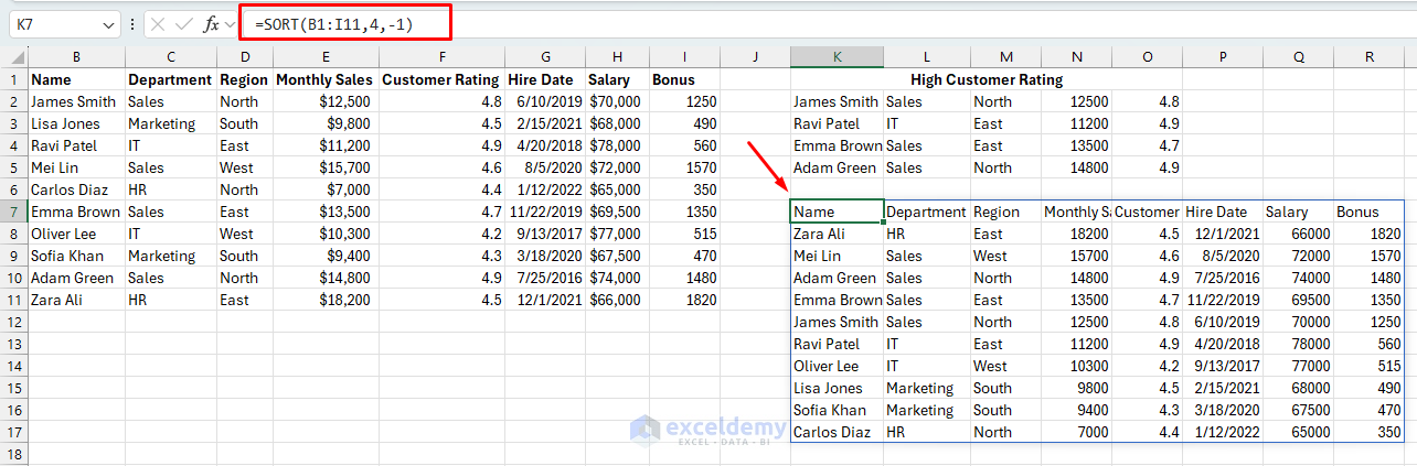

SEQUENCE

Generate a sequence for Employee IDs:

=SEQUENCE(10,1,101,1)

This formula generates an employed ID starting from 101.

Combine Dynamic Array Functions:

You can combine dynamic array functions to perform complex operations. Let’s find top performers from a particular region and sort them by sales:

=SORT(FILTER(A2:I11, (E2:E11>=12000)*(D2:D11="East")), 5, -1)

3. Power Query: ETL for Excel

Power Query (Get & Transform) brings enterprise-level ETL (Extract, Transform, Load) capabilities to Excel. It connects to various data sources, transforms data with a visual interface, and loads the results into Excel.

Combine Monthly Sales Reports

Consider you have separate Excel files with monthly sales data, each with slightly different formatting:

Power Query Solution:

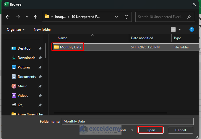
• Go to the Data tab >> from Get Data >> select From File >> select From Folder.

• Select the folder containing all files.

• You can select Combine & Load to directly load the data into the sheet.

• Preview the file to select the sample file.
• Click OK.

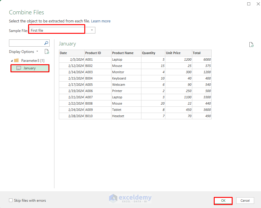
Output:

• You can select Combine & Transform Data to transform the data.
• In Power Query Editor:
  • Remove the source file.
  • Select the Source File column >> right-click>> select Remove.
  • Ensure data formats are consistent.
  • Remove any blank rows.
  • Format all currency values consistently.

Add Month Column From Date:

• Select the Date Column.
• Go to the Add Column tab >> from Date >> select Month >> select Name of Month.
• Adds a new column like January, February, etc.

Group by Product & Month:

• Select Product Name and Month columns (hold Ctrl)
• Go to the Home tab >> select Group By.
• In the Group By dialog box:
  • Group by: Product Name, Month
  • New column name: Total Sales
  • Operation: Sum
  • Column: Total
• Click OK.

• You will get a summary table of total sales by product and by month.
• Go to the Home tab >> select Close & Load To… to bring the grouped table back into Excel.

The result is a clean, consolidated dataset that combines all monthly files despite their formatting differences, ready for analysis in Excel.

4. Linked Data Types: Real-World Data in Your Spreadsheet

Excel’s linked data types connect cells to real-world entities and their associated data. It can transform text into rich data objects that can be queried for additional information.

Suppose you have sales data by country and want to enrich it with geographic information:

Steps to use Geography Data Type:

• Select cells containing country names.
• Go to the Data tab >> from Data Types >> select Geography.

• The country names convert to Geography data types (indicated by a small map icon).
• Insert geographic data from the Insert Data pane.

• Now you can extract geographic data using dot notation:

In the column D, add “Population”:

=A2.Population

Stock Data Type Example:

Similarly, create a portfolio tracker:

• Type stock symbols in the column.
• Select the stock symbols column.
• Go to the Data tab >> from Data Types >> select Stocks.
• You can use the Insert Data option, or you can use the formula.
• Use formulas like:

=A2.Price

5. LET Function: Simplify Complex Formulas

The LET function allows you to define named variables within a formula, making complex calculations more readable and efficient. Creates temporary named variables within a formula’s scoop.

Calculate adjusted Salary after bonus and tax deduction:

=LET(
base, H2,
bonus, I2,
tax, (base+bonus)*22%,
net_salary, base + bonus - tax,
net_salary
)

• This formula caluctes the Net Salary with payrool calculation, which is easily maintable.

Benefits:

• Makes complex formulas more readable
• Improves calculation efficiency by computing repeated expressions only once
• Keeps temporary variables contained within the formula
• Reduces errors by calculating intermediate values just once

6. Workbook Statistics: Understand Your Spreadsheet’s Complexity

Excel’s Workbook Statistics provides insights into your spreadsheet’s structure and complexity. It displays a comprehensive overview of your workbook’s elements.

Imagine you’ve inherited a complex financial model workbook from a colleague who has left the company. The file is massive, calculation-intensive, and runs slowly. Before attempting to optimize it, you need to understand its complexity.

Quickly analyze workbook complexity:

Access via:

• Go to the Review tab >> select Workbook Statistics.
• Instantly view total sheets, formulas, tables, and workbook size.
• Helps track complexity and manage efficiency.

Pro tip: Run Workbook Statistics before and after your optimization to quantify the improvements you’ve made in terms of complexity reduction.

7. Sheet View: Personalized Views Without Affecting Others

Sheet View allows multiple users to create personalized views of the same shared workbook without affecting what others see.

It enables individual sorting, filtering, and other changes without disrupting the main view.

Each team member needs to analyze different aspects of this data:

Region Manager View

• Open the shared workbook.
• Go to the View tab >> click Sheet View >> select New.
• Filter the Region column to show only East.
• Click Save View >> Name it EastRegionAnalysis.

Switch between views:

• On the View tab >> click Sheet View.
• Select the desired view from the dropdown menu.

Key Benefits:

• Each team member can analyze the data differently without affecting others.
• No need to create and maintain separate copies of the report.
• The original data remains intact and unchanged.
• Team members can share their views with specific colleagues.
• Everyone works from a single source of truth.

Pro tip: Use Sheet View to prepare multiple analysis scenarios for a meeting without creating separate files or sheets.

8. Custom Data Types: Define Your Data Structures

Custom data types allow you to define complex, structured data directly in Excel. It can create rich, reusable data structures with multiple properties.

Let’s create a Custom “Employee” data type:

Step 1: Load Data into Power Query

• Select your data range.
• Go to the Data tab >> click From Table/Range.
  • Make sure the data has headers.
  • Click OK to open Power Query Editor.

Step 2: Select and Structure Fields

• Select the Employee ID column.
• Go to the Home tab >> select Group By.
  • Group by Employee ID (or Name if IDs aren’t unique).
  • Name the column: Employee.
  • Use All Rows as the operation.
  • This nests the selected fields into a record/table.

Step 3: Create Data Type

• Click the expand icon (⤢) next to the EmployeeDetails column.
• You’ll see a dropdown: select all fields (Name, Department, etc.)
• Uncheck Use original column name as prefix for cleaner names.
• Click OK.

• Now you’ll see all the individual fields (columns) like Name, Department, Region, etc., next to Employee ID.
• Go to the Transform tab >> select all fields except Employee ID.
• Right-click >> select Create Data Type.
• In the Create Data Type dialog:
  • Select Advanced display.
  • Data type name: Employee.
  • Display column: Name (or any field you want to show).
  • Selected columns: All fields you want in the data type.
• Click OK.

• Click Close & Load To…
  • Choose Table or Only Create Connection (if you’ll use it elsewhere).

Step 4: Use Custom Data Type in Excel

Now you’ll see a single column with cells containing [Record].

• Click the Insert Data >> select the fields.
  • Department
  • Salary
  • Hire Date
  • Region
  • Custom Rating
  • Monthly Sales

Or use formulas like:

= [@Employee][Salary]

This keeps your main table clean while still allowing access to rich, structured data.

9. Excel JavaScript API: Automate Excel in the Cloud

The Excel JavaScript API enables developers to create add-ins that interact with Excel content. It provides programmatic access to Excel objects in web and desktop versions. The Excel JavaScript API enables developers to create add-ins that interact with Excel content.

Key capabilities:

• Create custom functions.
• Manipulate worksheets, ranges, tables, and charts.
• Build custom interfaces in the task pane.
• Automate workflows across Microsoft 365.
• Integrate with external data sources and web services.

Example use case: Create a custom add-in that pulls data from your company’s API, processes it according to business rules, and updates specific worksheets.

10. Live Collaboration Tools: Real-Time Teamwork

Excel’s live collaboration features transform spreadsheets from individual tools to team workspaces. Multiple users can work on the same workbook simultaneously.

Steps:

• Upload the file to OneDrive/SharePoint.
• Select Share >> Invite team members.
• Simultaneously update data, leave comments, and view changes instantly.

Key collaboration features:

• Real-time co-authoring in Excel Online and desktop versions.
• Comments and @mentions for contextual discussions.
• Version history to track changes.
• Shared workbook notifications.
• Status bar indicators show who’s working where.

Pro tip: Use comments with @mentions to assign tasks or request input from team members on specific cells or ranges.

Conclusion

These ten unexpected features unlock Excel’s hidden potential, automate complex tasks, and enhance productivity. By mastering these capabilities, you can transform your data workflows, automate complex tasks, and collaborate more effectively with your team. These features are helpful for financial analysts, data scientists, business managers, or just Excel enthusiasts.