10 Excel Formulas Every Non-Power User Ends Up Googling

 

Excel formulas can be tricky for new and even regular users, but some formulas come up so often that nearly everyone finds themselves searching for them. Many users have stared at a spreadsheet, knowing Excel can do what they need, but not quite remembering the syntax.

In this tutorial, we will cover 10 Excel formulas every non-power user ends up Googling. To demonstrate the practical use of these formulas, we’ll use a sample sales dataset.

1. SUMIF – Adding with Conditions

Usually, users are familiar with the SUM function, which adds up a range of numbers. However, the SUMIF function calculates the sum of values that meet specific criteria.

Syntax:

=SUMIF(range, criteria, [sum_range])

Let’s calculate total sales for a specific region.

• Select a cell and insert the following formula.

Formula:

=SUMIF(C2:C21, "North",G2:G21)

This formula calculates the total sales amount for the North region.

Common Uses:

• Sum values greater than 100: =SUMIF(F2:F21, “>100”)
• Sum based on partial text match: =SUMIF(A:A, “*Laptop*”, B:B)

Asterisks are wildcards; *Laptop* finds any cell containing “Laptop” anywhere in the text.

2. MIN/MAX & AVERAGE – Track Performance

While maintaining sales data, you’ll often need to find the minimum, maximum, and average sales to track performance.

Syntax:

=MIN(Number1, [Number2],..) - Returns the smallest value

=MAX(Number1, [Number2],..) - Returns the largest value

=AVERAGE(Number1, [Number2],..) - Calculates the arithmetic mean of a group of numbers

MIN:

• Find out the lowest sales amount.

Formula:

=MIN(G2:G21)

MAX:

• Show the highest sales amount.

Formula:

=MAX(G2:G21)

AVERAGE:

• Calculate the average sales amount.

Formula:

=AVERAGE(G2:G21)

These functions are used to track overall sales performance.

3. IF Statements – Making Decisions

The IF function performs different actions based on whether a condition is true or false. You can use this function to categorize, flag, or add logic to your data.

Syntax:

=IF(logical_test, value_if_true, value_if_false)

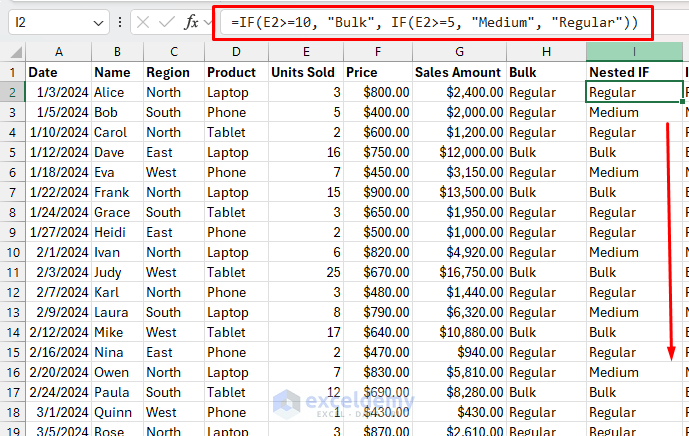
Let’s mark sales as ‘Bulk’ if the units sold are 10 or more.

• Select a cell and insert the following formula.

Formula:

=IF(E2>=10, "Bulk", "Regular")

This formula automatically categorizes each sale based on the number of units sold.

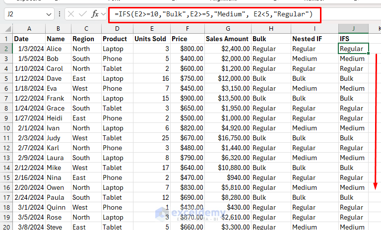
For Multiple Conditions:

You can use either the nested IF function or the IFS function to test multiple conditions.

=IF(E2>=10, "Bulk", IF(E2>=5, "Medium", "Regular"))

=IFS(E2>=10,"Bulk",E2>=5,"Medium", E2<5,"Regular")

Tip: You can nest up to 64 IF statements, but consider using other functions like SWITCH or IFS for complex logic.

4. COUNTIF – Counting with Conditions

While the COUNT function is straightforward for counting cells with numbers, users often need to Google how to count cells that meet a specific criterion. This is where COUNTIF comes in.

Syntax:

=COUNTIF(range, criteria)

Let’s count sales of $10,000 or more.

• Select a cell and insert the following formula.

Formula:

=COUNTIF(G2:G21, ">=10000")

This formula counts how many individual sales were $10,000 or more.

Common Uses:

• Count specific text: =COUNTIF(A:A, “Complete”)
• Count cells that aren’t blank: =COUNTIF(A:A, “<>”)

COUNTIFS for Multiple Criteria:

If you want to count sales based on multiple criteria, you can use the COUNTIFS function.

=COUNTIFS(C2:C21, "North", G2:G21, ">=10000")

This counts rows where column C is “North” AND column G is greater than or equal to 10000.

5. VLOOKUP – Finding Data in Another Table

VLOOKUP is one of the most popular formulas for searching for values in a table. It searches for a value in the first column of a table and returns a value from another column in the same row.

Syntax:

=VLOOKUP(lookup_value, table_array, col_index_num, [range_lookup])

Let’s find the price of a Tablet.

• Select a cell and insert the following formula.

Formula:

=VLOOKUP("Tablet", D2:G21, 3, FALSE)

This formula searches for the Tablet price and returns the price from the table.

• “Tablet” is what we’re looking for.
• D2:G21 is our lookup table.
• 3 means retrieve the value from the 3rd column of the table array (Price).
• FALSE means exact match only.

Common Mistake: Forgetting that VLOOKUP can only look to the right; it searches in the leftmost column of the table and returns values from columns to its right.

6. CONCATENATE/TEXTJOIN (or the & operator) – Combining Text

These functions are helpful for joining values from multiple cells.

CONCATENATE:

The CONCATENATE function joins text from multiple cells into one cell.

Let’s combine the first and last names to get the full name.

• Select a cell and insert the following formula.

Formula:

=CONCATENATE(A2, " ", B2)

This formula returns the full name.

Ampersand Operator:

You can use the ampersand (&) operator to join cell values. You don’t need a function for this.

Formula:

=A2 & " " & B2

This formula combines the first and last names and returns the full name.

TEXTJOIN:

Excel 365 users can use CONCAT or TEXTJOIN for more flexibility.

• Let’s join the Department and Employee ID.

=TEXTJOIN("-", TRUE, C2, D2)

=CONCAT(C2, "-", D2)

7. LEFT, RIGHT, MID – Extracting Parts of Text

When exporting data from various sources, users often need to extract specific portions of text strings.

Syntax:

=LEFT(text, num_chars) – Extracts characters from the left
=RIGHT(text, num_chars) – Extracts characters from the right
=MID(text, start_num, num_chars) – Extracts characters from the middle

LEFT:

• Let’s extract the product type from the Product Code.

Formula:

=LEFT(A2, 3)

This formula extracts the first 3 characters from the product code, which represent the product type.

RIGHT:

• Let’s get the Order Number from the Order ID.

Formula:

=RIGHT(C2, 4)

This formula extracts the last 4 characters, which represent the order number.

MID:

• Let’s extract the year from the Product Code.

Formula:

=MID(A2, 5, 2)

This formula extracts two characters starting from the 5th position, which represents the year.

Common Use: Extracting area codes, splitting product codes, or parsing imported data.

8. TRIM – Cleaning Up Messy Data

When importing data from other systems, you often get messy text with random spaces that break formulas and lookups. The TRIM function removes all extra spaces from text, including leading, trailing, and multiple spaces between words.

Syntax:

=TRIM(text)

Let’s use TRIM to clean up names with leading and trailing spaces.

• Select a cell and insert the following formula.

Formula:

=TRIM(A2)

This formula removes the unnecessary spaces from the names.

Tip: Always use TRIM on imported data before using it in VLOOKUP or other formulas.

9. TODAY and NOW – Current Date and Time

Excel offers dynamic date and time functions, which are helpful for timestamps, calculating deadlines, or tracking progress.

Syntax:

• TODAY() – returns today’s date
• NOW() – returns the current date and time

TODAY:

• Select a cell and insert the TODAY function.

=TODAY()

This formula shows the current date and updates every time Excel recalculates.

NOW:

• Select a cell and insert the NOW function.

=NOW()

This formula shows a timestamp that also updates dynamically.

Important Note: These functions update automatically. If you need a static date, type the date manually or use Ctrl+; for the current date.

10. IFERROR – Handling Formula Errors Gracefully

The IFERROR function replaces ugly error messages with something more user-friendly.

Syntax:

=IFERROR(value, value_if_error)

Instead of showing #N/A when VLOOKUP fails, you can display a custom message instead.

Formula:

=IFERROR(VLOOKUP("Mouse", D2:G21, 3, FALSE), "Not Found")

If ‘Mouse’ is not found in the table, this formula will display ‘Not Found’ instead of an error.

Common Errors This Fixes:

• #N/A (VLOOKUP couldn’t find the value).
• #DIV/0! (dividing by zero).
• #VALUE! (wrong data type).

Bonus Tips for Excel Success

• Use Absolute References When Copying Formulas:
  • $A$2 remains $A$2 when copied.
  • A2 changes to A3, A4, etc. when copied down.
  • $A2 keeps the column absolute but allows the row to change.
• Use Named Ranges:
  • Instead of =SUMIF(Sheet2!A:A, “North”, Sheet2!B:B),
  • Create named ranges: =SUMIF(Regions, “North”, Sales)
• Use Ctrl+Shift+Enter for Array Formulas:
  • Some advanced formulas need this to work properly (you’ll see curly braces {} appear).
• F4 Toggles Reference Types:
  • Select a cell reference in a formula and press F4 to cycle through A1, $A$1, A$1, and $A1.

Final Thoughts

These ten are commonly used formulas that every user should know. Mastering these formulas will make your spreadsheets more powerful and save you a lot of time searching for help online. It will reduce your Google searches and give you more confidence in tackling common Excel tasks. Try using each formula in your workbook, modify the examples, and get comfortable with how they work.