What Is Yield to Maturity?
Yield to Maturity is the measure of the total return where the bond is held for a maturing period. We can express it as an annual rate of return. It is also known as Book Yield or Redemption Yield. It is different from the Current Yield as it takes into account the present value of a future bond.
Yield to Maturity Formula
You can use the formula below to calculate the Yield to Maturity value:
YTM=(C+(FV-PV)/n)/(FV+PV/2)
C= Annual Coupon Amount
FV= Face Value
PV= Present Value
n= Years to Maturity
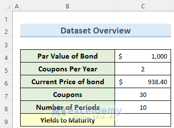
The sample dataset contains 6 rows and 2 columns. Cells contain dollars in Accounting format and in Percentage format.
Method 1 – Using the RATE Function
The RATE function will be used.
Steps:
- Go to C9 and insert the following formula:
=RATE(C8,C7,-C6,C4)*C5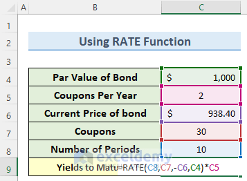
- Press Enter to calculate the Yields to Maturity value in percentage.

Read More: How to Calculate Coupon Rate in Excel
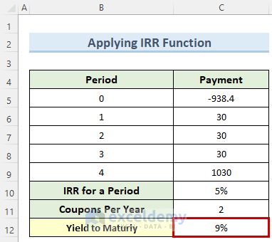
Method 2 – Applying the IRR Function
The IRR function will be used.
Steps:
- Double-click C10 and enter the formula:
=IRR(C5:C9)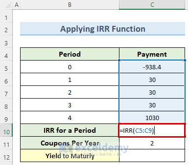
- Press Enter to get the IRR value for a period.
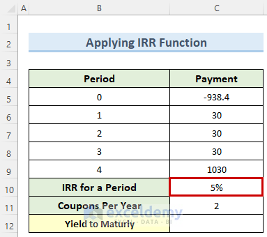
- Go C12 and use the formula below:
=C10*C11
- Press Enter to see the Yield to Maturity value in C12.
Read More: Calculate Price of a Semi Annual Coupon Bond in Excel
Method 3 – Utilizing the YIELD Function
The YIELD function will be used.
Steps:
- Double-click C11 and enter the formula below:
=YIELD(C6,C7,C5,C10,C4,C8)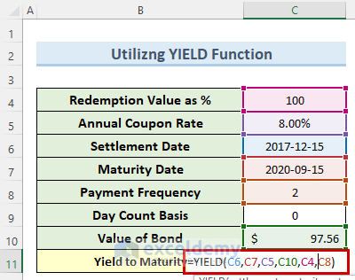
- Press Enter and find the Yield to Maturity value in C11.

Read More: Calculate Bond Price from Yield in Excel
Method 4 – Calculating the Yield to Maturity by using a Direct Formula
Steps:
- In C8, enter the following formula:
=(C6+((C4-C5)/C7))/(C4+C5/2)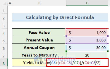
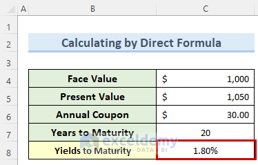
- Press Enter or click any blank cell.
- The percentage value of the Yield to Maturity will be displayed.
Read More: Calculate Bond Price with Negative Yield in Excel
Things to Remember
- Remember to add a ‘-’ sign before C6 inside the RATE function.
- You might see a #NUM! error if you forget the negative sign.
- If you insert any non-numeric data, you will get a #VALUE! error.
- The arguments in the IRR function must have at least one positive and one negative value.
- The IRR function ignores empty cells and text values.
Download Free Calculator
You can download the free calculator here.
Related Articles
- How to Calculate Clean Price of a Bond in Excel
- Calculate Face Value of a Bond in Excel
- Calculate the Issue Price of a Bond in Excel
- Calculate Duration of a Bond in Excel
- How to Calculate Bond Payments in Excel
- How to Calculate Present Value of a Bond in Excel
- Compute Floating Rate Bond Valuation in Excel
<< Go Back to Bond Price Formula Excel|Excel Formulas for Finance|Excel for Finance|Learn Excel
Get FREE Advanced Excel Exercises with Solutions!

This is a great work, clear and easy to understand.
Thanks
Great work. Thanks for sharing
Nice to hear that you found this article helpful. Thanks for the feedback!
Best regards
Great job will put all templates to work,
how ever looking for template for my “Dividend Tracking Portfolio” of 5~6 k with very few MANUAL entry love to download free if available or for reasonable price. keep up good work
I have a puzzling situation
Rate function does not work for some combination of numbers.
For example:
PV = -890
FV = 1000
pmt = 200
Nper = 31
There are other combinations too The answer is #NUM!
Any help?
Hi GABRIEL!
Thank you for your comment.
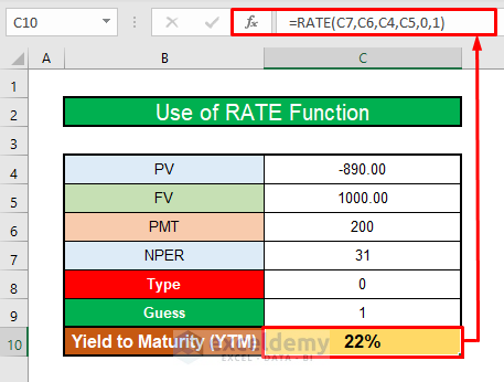
The RATE function does not work for some combinations. In these cases, the #NUM! error occurs. To solve this error simply add the Type and the Guess arguments in the RATE function. For Type, 0 or omitted is used for at the end of the period and 1 is used for at the beginning of the period. If RATE does not converge, try different values for the guess. RATE usually converges if the guess is between 0 and 1.
Using these two arguments, you can solve the #NUM! Error. Look at the below screenshot.
Please download the Excel file for your practice.
https://www.exceldemy.com/wp-content/uploads/2022/09/Calculate-Yield-to-Maturity.xlsx
Regards
Md. Abdur Rahim Rasel (Exceldemy Team)
I don’t understand your YTM premise. Its a 10 year bond, two coupons per year, and you input 30 coupons? Something is missing or I am missing something. Thanks in advance.
Hello Bruce,
Thank you for your feedback and for pointing out the error. In this case, instead of Coupons it should be Coupon Payment which in this case has been considered $30.0 as shown in the updated picture below.
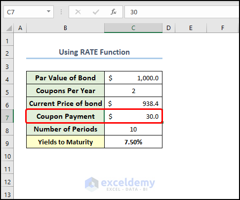
Hopefully, this clears out any confusion and we are sorry for this error.
Regards,
ExcelDemy