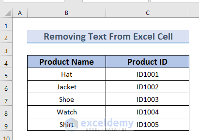
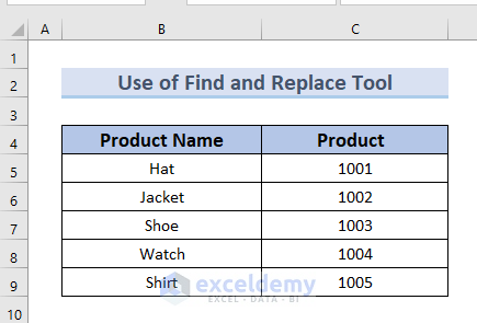
In the following dataset, you can see the Product Name and Product ID columns. Let’s use it to demonstrate how you can remove text from the IDs.
Method 1 – Using Find and Replace Tool to Remove Text from a Cell in Excel
Steps:
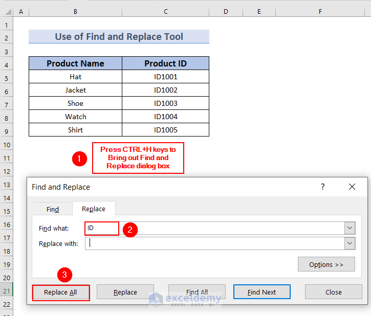
- Click Ctrl + H to open the Find and Replace dialog box.
- Write ID in the Find what. Leave the Replace with box empty.
- Press Replace All.
- Click OK in the notification box.
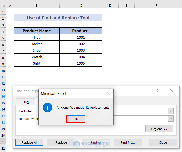
- The text ID has been removed from all the cells (including the header).
Read More: How to Remove Text from an Excel Cell but Leave Numbers
Method 2 – Use of SUBSTITUTE Function to Remove Text from a Cell
Steps:
- Type the following formula in cell D5:
=SUBSTITUTE(C5,”ID”,””)
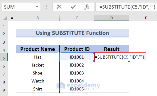
- Press Enter.
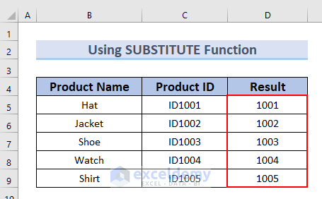
- Copy the formula to the other cells using the Fill Handle.
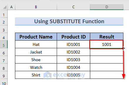
- The Result column autofills:
Read More: How to Remove Letters from Cell in Excel
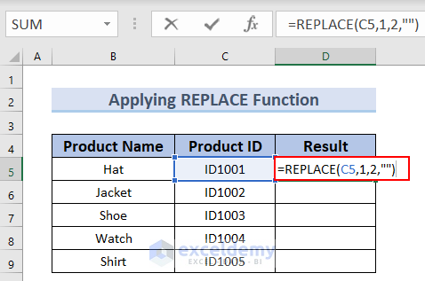
Method 3 – Applying REPLACE Function to Remove Text from a Cell in Excel
Steps:
- Write the formula in cell D5 as given below:
=REPLACE(C5,1,2,””)
- Press Enter.
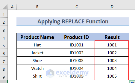
- Drag down the formula with the Fill Handle tool.

You can see the complete Result column.
Read More: How to Remove Specific Text from Cell in Excel
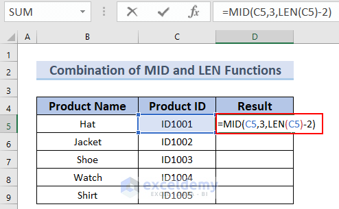
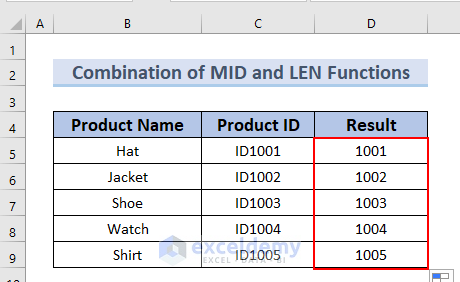
Method 4 – Combining MID and LEN Functions
The LEN function is a text function in excel that returns the length of a string/ text.
Steps:
- Select cell D5.
- Copy this formula:
=MID(C5,3,LEN(C5)-2)
Formula Breakdown
- LEN(C5) → becomes
- LEN(“ID1001”)
- Output: 6
- LEN(“ID1001”)
- LEN(C5)-2 → becomes
- LEN(6-2)
- Output: 4
- LEN(6-2)
- MID(C5,3,LEN(C5)-2) → becomes
- MID(“ID1001”,3,4)
- Output: 1001
- MID(“ID1001”,3,4)
- Press Enter.
- Drag down the formula with the Fill Handle tool.
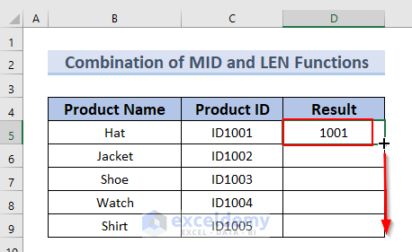
You can see the complete Result.
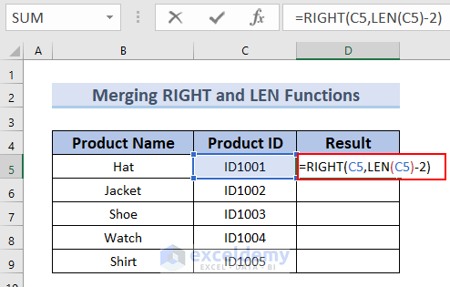
Method 6 – Merging RIGHT and LEN Functions
Steps:
- In cell D5, type the given formula:
=RIGHT(C5,LEN(C5)-2)
Formula Breakdown
- LEN(C5) → becomes
- LEN(“ID1001”)
- Output: 6
- LEN(“ID1001”)
- LEN(C5)-2 → becomes
- LEN(6-2)
- Output: 4
- LEN(6-2)
- RIGHT(C5,LEN(C5)-2) → becomes
- RIGHT(“ID1001”,4)
- Output: 1001
- RIGHT(“ID1001”,4)
- Press Enter.
- Drag down the formula with the Fill Handle tool.
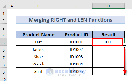
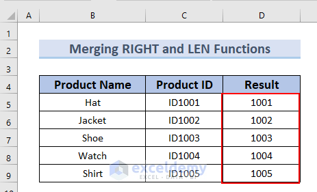
You can see the complete Result column.
Read More: How to Remove Text before a Space with Excel Formula
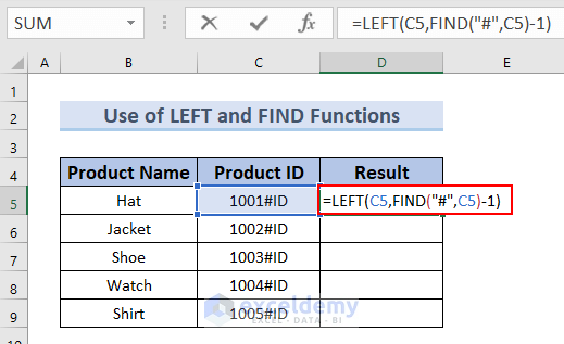
Method 6 – Using LEFT and FIND Functions to Remove Text from a Cell in Excel
We have rearranged the dataset to include more characters. Let’s remove the characters before and including ‘#’ from every cell.
Steps:
- Select cell D5 and write the formula given below:
=LEFT(C5,FIND(“#”,C5)-1)
Formula Breakdown
- FIND(“#”, C5) → The FIND function will find the position of ‘#’ in cell C5.
- Output: 5
- LEFT(C5, FIND(“#”, C5)-1) → We have subtracted 1 because we want to remove the ‘#’ too. Then the LEFT function will keep the number of characters from the left side.
- Output: 1001
- Press Enter.
- Drag down the formula with the Fill Handle tool.
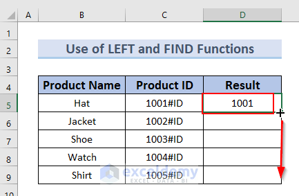
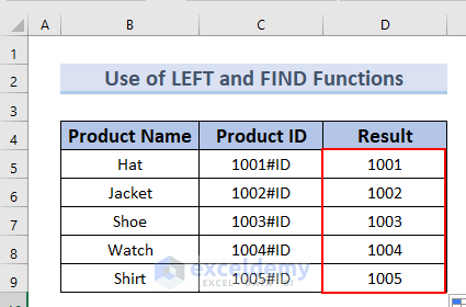
You can see the complete Result column.
Read More: How to Remove Text After Character in Excel
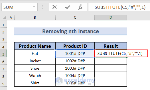
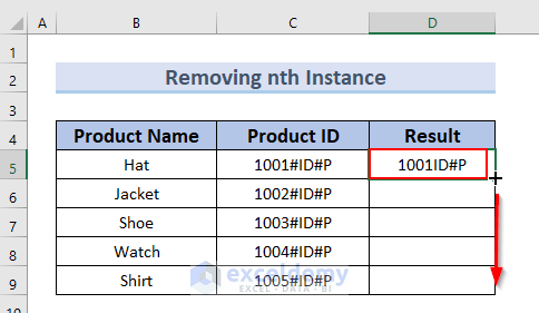
Method 7 – Removing Nth Instance of Certain Character
We have rearranged my dataset to have two ‘#’ in every cell. We’ll remove the first ‘#’.
Steps:
- Select cell D5 and type the formula given below:
=SUBSTITUTE(C5,”#”,””,1)
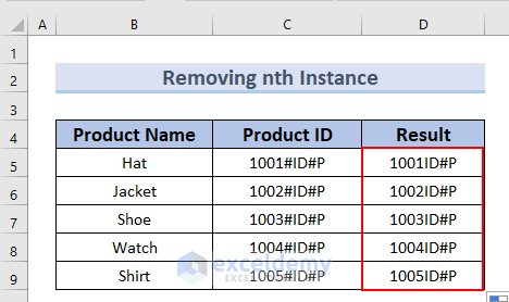
- Hit Enter.
- Copy the formula for the other cells with the AutoFill feature.
You can see the complete Result column.
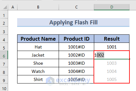
Method 8 – Applying Flash Fill Feature
Steps:
- Type the digits you want to keep in cell D5.
- When you start typing in the next cell, Excel will catch the pattern and show it.
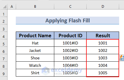
- Press Enter and all cells will be filled with that pattern.
Read More: How to Remove Text between Two Characters in Excel
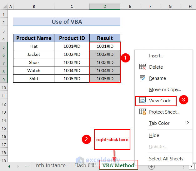
Method 9 – Using VBA Code to Remove Text from a Cell
Steps
- Select the cell range to apply VBA. We selected cells D5:D9.
- Right-click on the title name of the sheet.
- Select View Code from the context menu.
- A VBA window will open up.
- Copy the code given below:
Sub Delete_Last_Char()
n = Int(InputBox("Type Number of Last Characters tobe Removed: "))
For i = 1 To Selection.Rows.Count
   Selection.Cells(i, 1) = Left(Selection. Cells(i, 1), _
   Len(Selection. Cells(i, 1)) - n)
Next i
End Sub 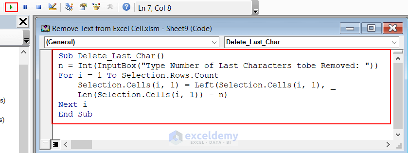
- Click the Run button to run the code.
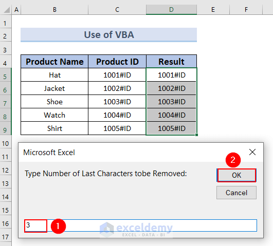
- An input window will appear. Type the number of characters that you want to remove. We typed 3.
- Press OK.
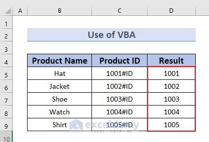
Therefore, the last 3 characters in the Result column are removed.
Read More: How to Remove Specific Text from a Column in Excel
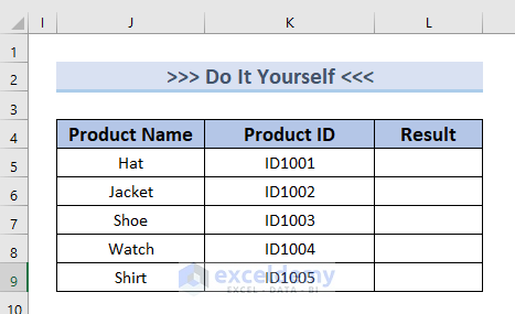
Practice Section
You can download the above Excel file and practice the explained methods.