How to Remove Specific Text from Cell in Excel (Easiest 11 Ways)

The following image shows an overview of removing specific text from cells in Excel.

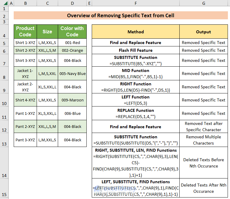
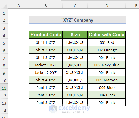
We have a dataset with 3 columns. We will remove specific string values from these cells based on various criteria.

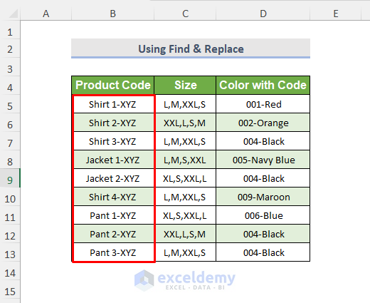
Method 1 – Using the Find and Replace Option to Remove a Specific Text from Cells in Excel

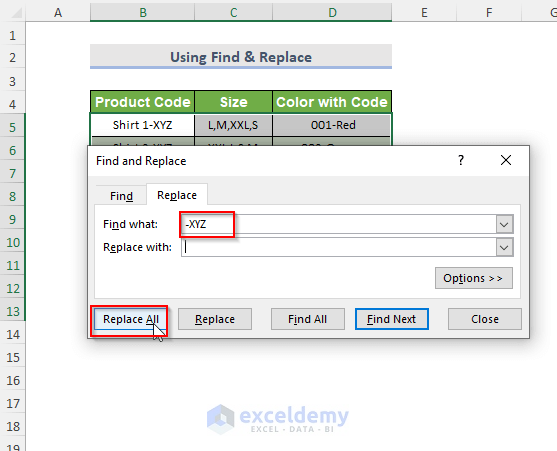
We will remove the ending “-XYZ” string from Product Code cells.

Steps:

Select the data table
Go to the Home tab and select Editing.
Choose Find & Select and click Find.

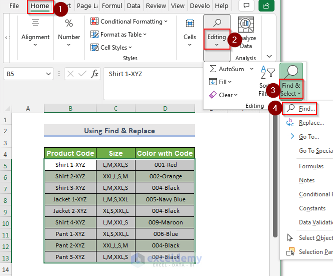
The Find and Replace dialog box will pop up.
Write -XYZ in Find What.
Keep Replace blank.
Select Replace All.

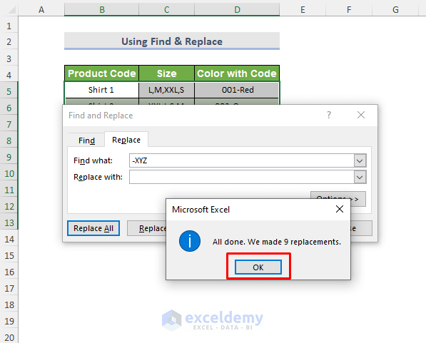
You’ll get a notification about the number of replacements. Click OK.

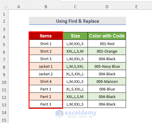
Here’s the result.

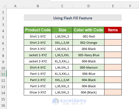
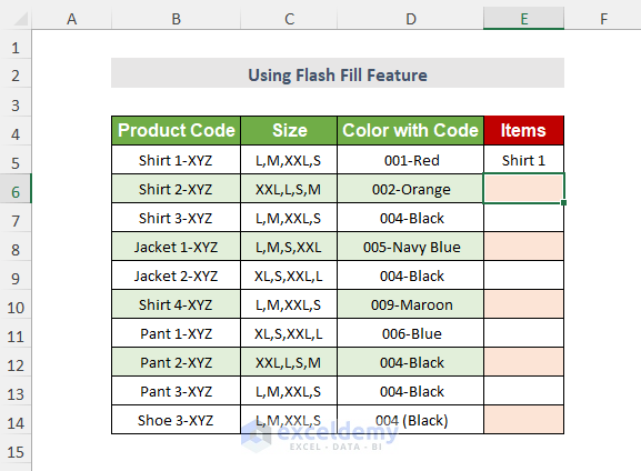
Method 2 – Removing Text from Cell with Flash Fill

We will extract the product name before the dash and extract it in a separate Items column.

Steps:

Write down the part of the text you want to keep in Cell E5.

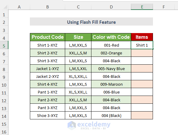
Press Enter.

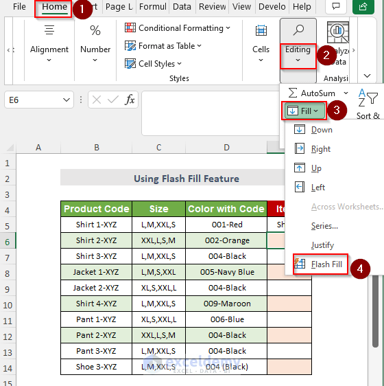
Go to the Home tab.
Select Editing, then Fill, and choose Flash Fill.

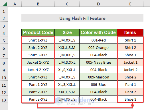
Here’s the output.

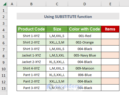
Method 3 – Using the SUBSTITUTE Function to Remove Specific Text from Cells

We’ll remove the “-XYZ” part from Product Code cells and extract the rest in the Items column.

Steps:

Select Cell E5.
Insert the following formula

=SUBSTITUTE(B5,"-XYZ","")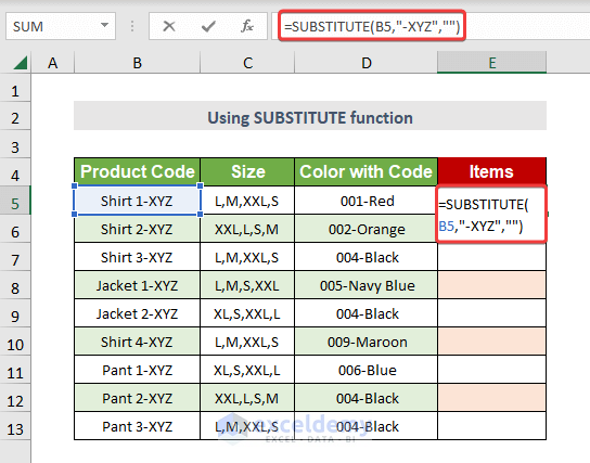

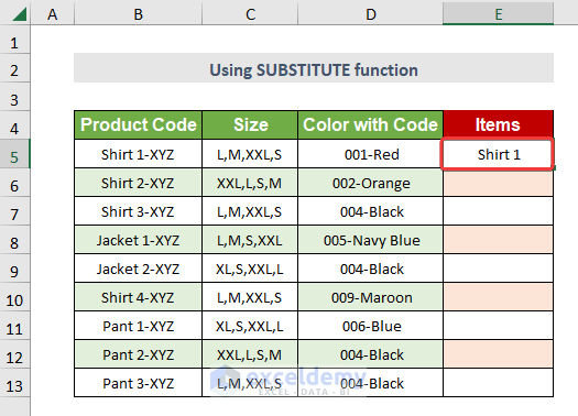
Press Enter.
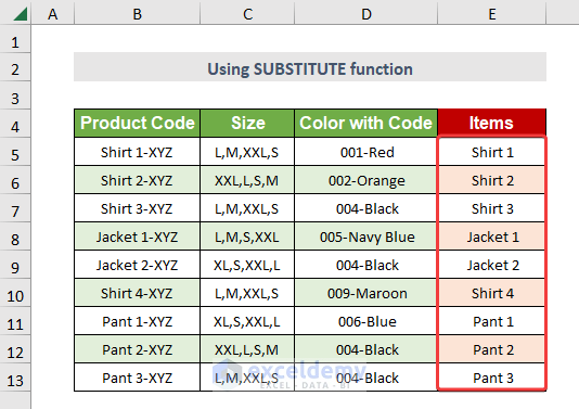
Drag down the Fill Handle tool.

Here’s the result.

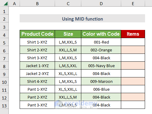
Method 4 – Applying the MID Function to Delete Specific Text from Cells

We’ll get the product names from the product code cells and put them in Items.

Steps:

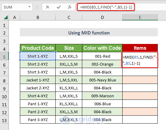
Select Cell E5.
Insert the following formula.

=MID(B5,1,FIND("-",B5,1)-1)

The FIND function finds the first dash in the B5 cell and returns its location. The MID function extracts the characters from the 1st character to that location from B5.

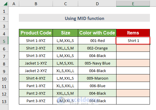
Press Enter.
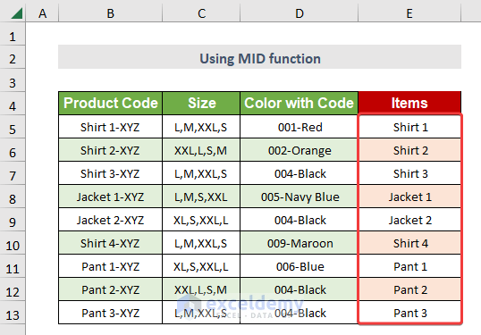
Drag down the Fill Handle tool.

You will get your desired result in the Items column.

Method 5 – Inserting the RIGHT Function to Remove Specific Text from Cells

In the Color with Code column, we have some colors combined with their code number. We’ll remove the code and the dash.

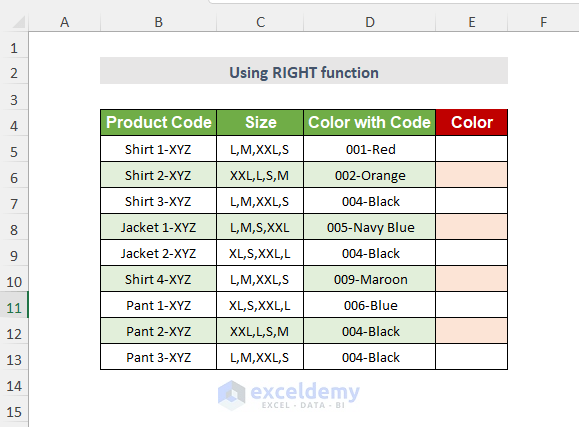
Steps:

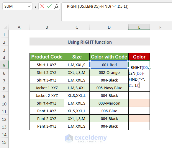
Select Cell E5.
Use the following formula.

=RIGHT(D5,LEN(D5)-FIND("-",D5,1))

D5 is the text,
LEN(D5) is the total length of the string
FIND("-", D5,1) will give the position of character “-” and then the value will be deducted from the total length of the string and it will be the number of characters for the RIGHT function.

Press Enter.
Drag down the Fill Handle tool.

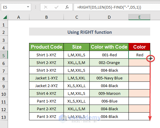
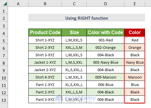
You will get only the names of the colors as below.

Method 6 – Applying the LEFT Function to Remove Text from Cells

We want to extract the Color Codes.

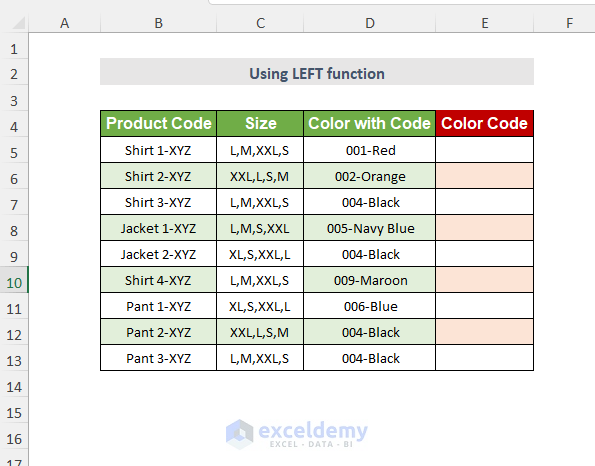
Steps:

Select Cell E5.
Insert the following formula.

=LEFT(D5,3)

D5 is the text,
3 is the number of characters you want to extract.

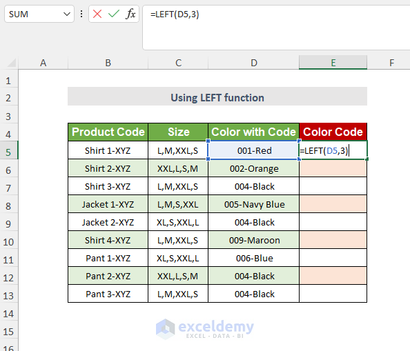
Press Enter.
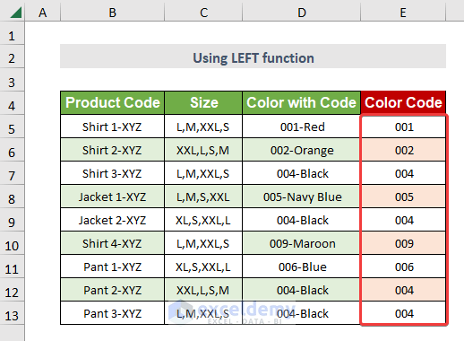
Drag down the Fill Handle tool.

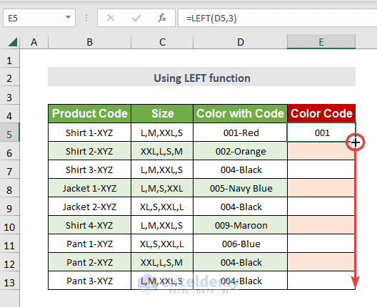
You will get the codes of colors in the Color Code column.

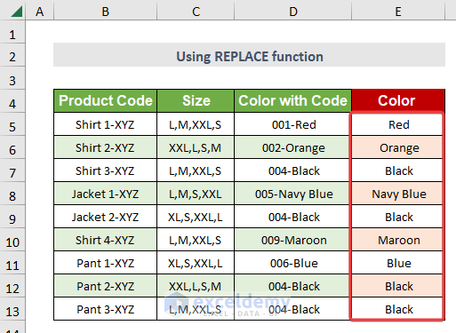
Method 7 – Using the REPLACE Function to Remove Text from Cells

We’ll remove the color codes from the color section and insert the results in the added the Color column.

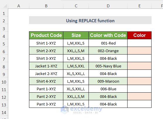
Steps:

Select Cell E5.
Insert the following formula:

=REPLACE(D5,1,4,"")

D5 is the text,
1 is the start number, 4 is the number of characters you want to replace with blank.

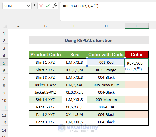
Press Enter.
Drag down the Fill Handle tool.

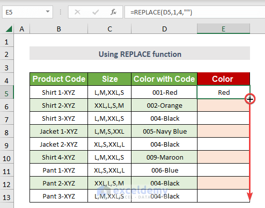
You will get the names of colors in the Color column.

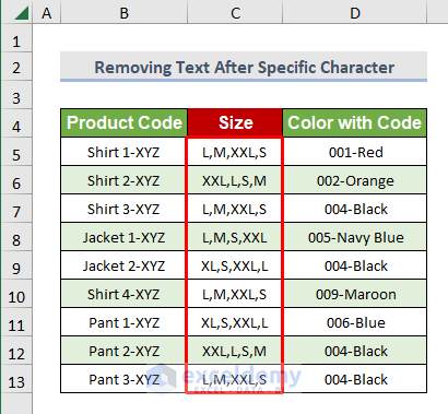
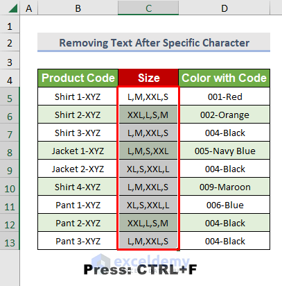
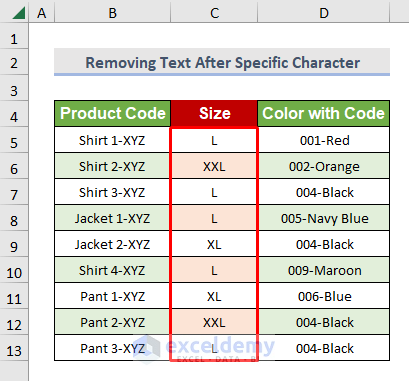
Method 8 – Removing Text After a Specific Character in Excel with Find and Replace

We want to remove the last three sizes in the Size column.

Steps:

Select the data table.
Go to Home, then to Editing, choose Find & Select, and click on Replace.

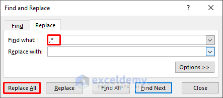
The Find and Replace dialog box will appear.
Write “,*” in the Find What box.
Keep the Replace with box empty.
Select Replace All.

Click OK on the notification.

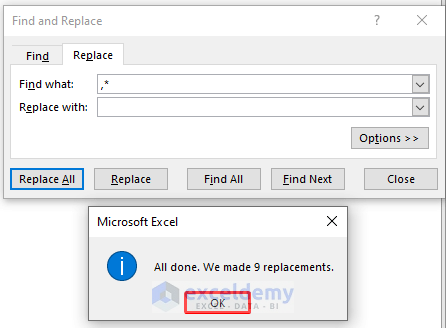
Click on Close and you can see the results.

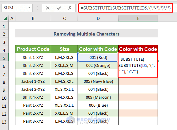
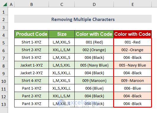
Method 9 – Removing Multiple Characters Simultaneously with SUBSTITUTE

We want to remove all of the brackets separating colors in the Color with Code column and use “-” as a separator.

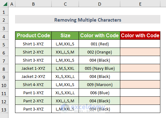
Steps:

Select Cell E5.
Insert the following formula:

=SUBSTITUTE(SUBSTITUTE(D5,"(","-"),")","")

D5 is the text,
SUBSTITUTE(D5,"(","-") here,“(” is the old text you want to replace with “-“.
This output will be used by another SUBSTITUTE function.

Press Enter.
Drag down the Fill Handle tool.

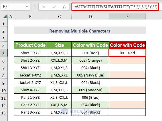
You will get your desired format in the output column as below.

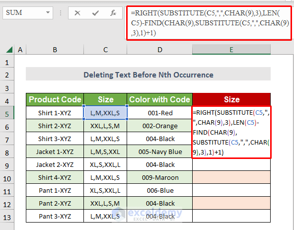
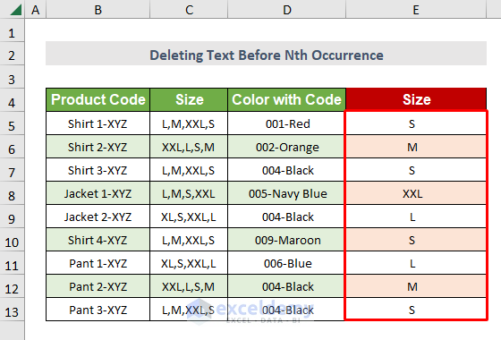
Method 10 – Deleting Texts before the N-th Occurrence of a Specific Character with RIGHT and SUBSTITUTE

We want to get only the last size instead of the 4 sizes in the Size column.

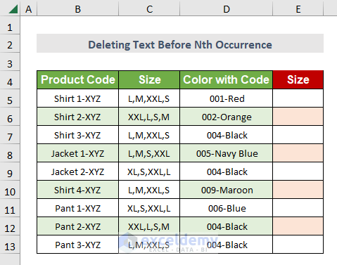
Steps:

Select Cell E5.
Insert the following formula:

=RIGHT(SUBSTITUTE(C5,",",CHAR(9),3),LEN(C5)-FIND(CHAR(9),SUBSTITUTE(C5,",",CHAR(9),3),1)+1)

C5 is the text,
SUBSTITUTE(C5,",", CHAR(9),3) here comma will be replaced by CHAR(9)(blank) and 3 is used to define the position of a comma before which I want to remove texts
The RIGHT function will give the output as the last size number from the right side.

Press Enter.
Drag down the Fill Handle tool.

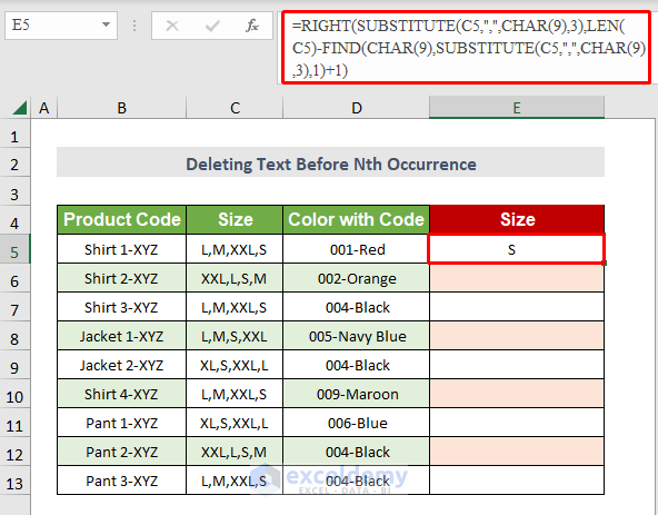
Here are the results.

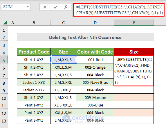
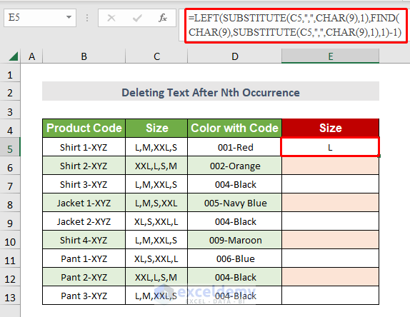
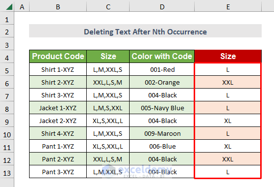
Method 11 – Removing Texts after the Nth Occurrence of a Specific Character Using LEFT and SUBSTITUTE

We’ll get only the first size.

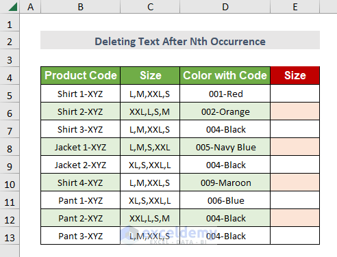
Steps

Select Cell E5.
Insert the following formula:

=LEFT(SUBSTITUTE(C5,",",CHAR(9),1),FIND(CHAR(9),SUBSTITUTE(C5,",",CHAR(9),1),1)-1)

C5 is the text,
SUBSTITUTE(C5,",", CHAR(9),3) here comma will be replaced by CHAR(9)(blank) and 1 is used to define the position of a comma after which I want to remove texts
The LEFT function will give the output as the last size number from the left side.