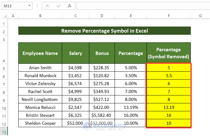
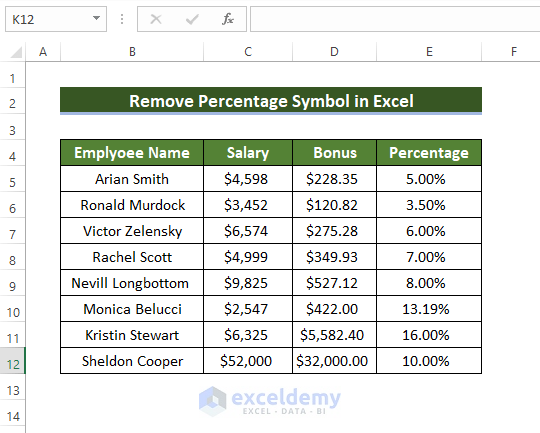
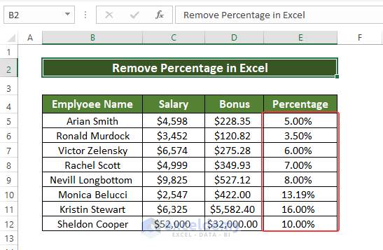
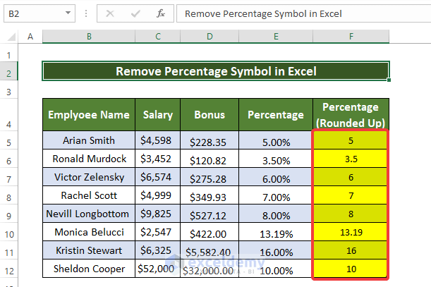
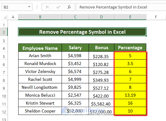
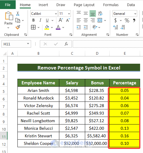
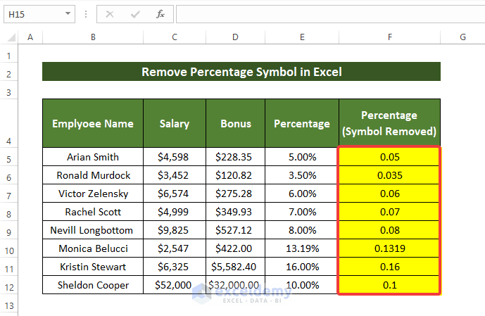
The dataset below will be used to demonstrate how to remove percentage symbols in Excel.
Method 1 – Use Custom Formatting to Remove the Percentage Symbol
Steps
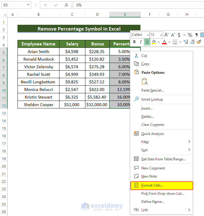
- Select the cells where you want to remove the percentage sign. We selected the range of cells E5:E12.
- Right-click and click Format Cells.
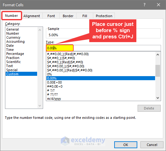
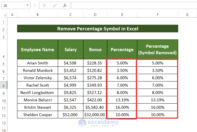
- In the format cells window, go to Number, then to Custom and, in the Type field, you will see 0.00% format.
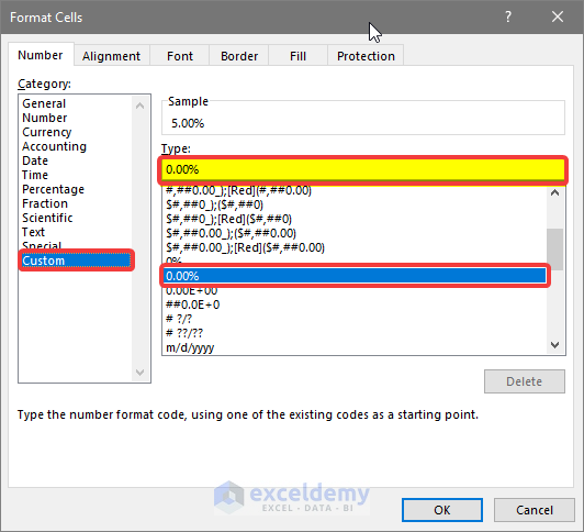
- In the Type field, place the cursor before the % sign and press Ctrl + J.
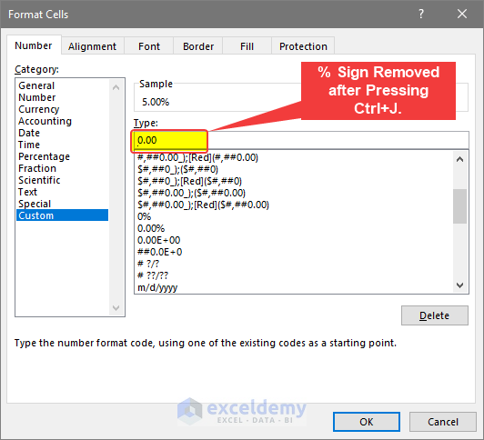
- The formatting in the Type field will change to 0.00. Click OK.
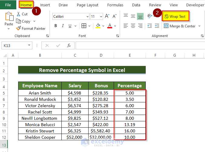
- The cells are still displaying the percentage symbols.
- To resolve this, select the range of cells E5:E12 again and click Wrap Text from the Home tab.
Read More: How to Remove Sign from Numbers in Excel
Method 2 – Using a Formula to Remove the Percentage Symbol
Steps
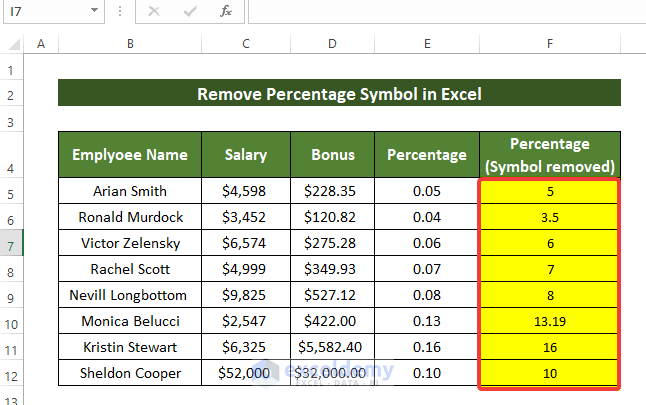
- Select cell F5 and enter the following formula:
=VALUE(LEFT(TEXT(E11,"000.0000%"),7))- The value in cell E5 is copied to cell F5 without the percentage symbol.
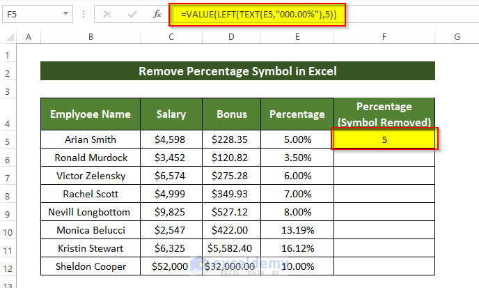
- Drag the fill handle icon down to apply the formula to the entire range of cells.

Breakdown of the Formula
1. TEXT(E8,”000.00%”): It takes the content in cell E8 as input and returns the text string in format 000.00.
2. LEFT(TEXT(E8,”000.00%”),5): This function will extract the 5 characters on the left side of the string return in TEXT function
3. VALUE(LEFT(TEXT(E8,”000.00%”),5)): This function will return the number from the string format from the left function.
Note:
You should enter the correct arguments inside the functions. The format 000.00 represents the rounding value, which is 2 here. You need to enter a suitable rounding value based on your own requirements.
Read More: Remove Percentage Symbol in Excel Without Changing Values
Method 3 – Applying Power Query in Excel
Steps
- Go to Data and select From Table/Range in Get and Transform Data group.
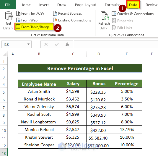
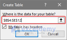
- A small window will open asking the range of the table.
- Select the range of cells B4:E12.
- Tick My table has headers to let Excel know that your table’s first row is the header.
- Click OK.
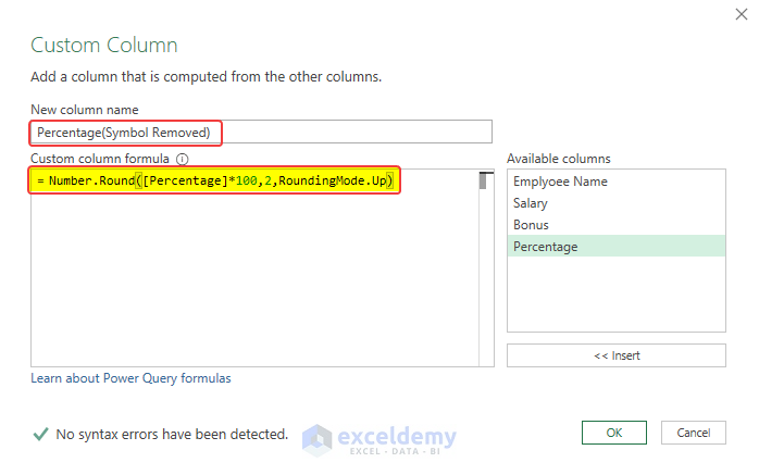
- A new window will open. Go to the Add Column tab and select Custom Column.
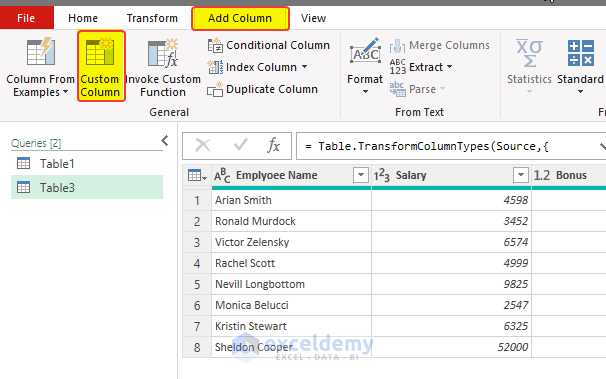
- A new options menu will appear. Enter a desired name in the New column name box.
- Enter the following formula in the Custom Column Formula field:
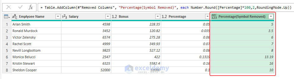
=Number.Round([Percentage]*100,2,RoundingMode.Up)- Click OK.
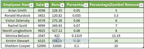
- A new column with all values from the Percentage column without the percentage symbol in the Percentage(Symbol Rounded) column will appear on the sheet.
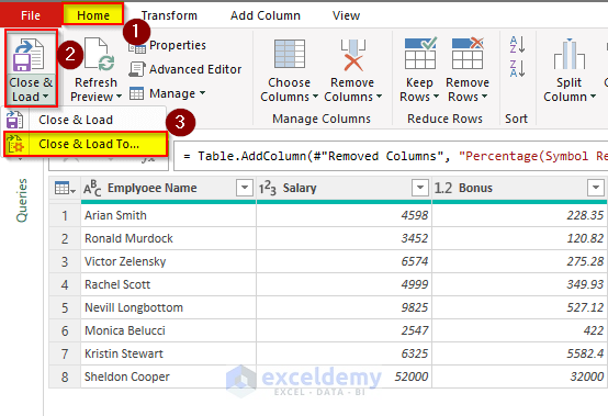
- Load these columns into the worksheet by clicking Close and Load.
- Select the option Close and Load To.
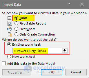
- The existing window will close and return to the main worksheet, with a new window.
- In that window, specify the location where you want to put the newly created table, select the location in the worksheet and click OK.
- The table created in the power query will now be in the worksheet with formatted percentage values.
- Copy the Percentage (Symbol Remove) column and paste it in the original table.
Read More: How to Remove Currency Symbol in Excel
Method 4 – Multiply with 100 to Remove the Percentage Symbol
Steps
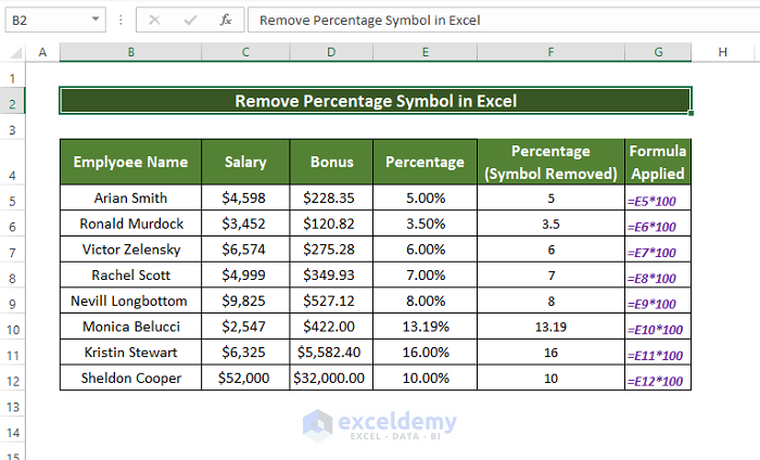
- Enter the following formula in cell F5:
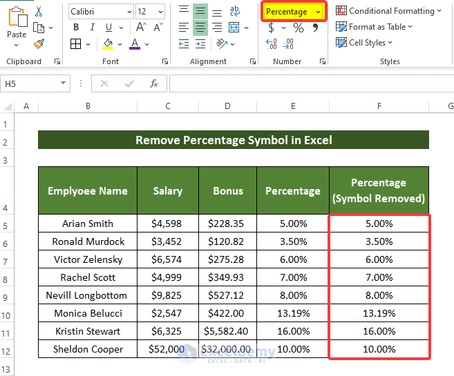
=E5*100- The values in the percentage column are displayed in the Percentage (Symbol Removed) column without the percentage sign.
Method 5 – VBA Macro to Remove Percentage Symbol
Steps
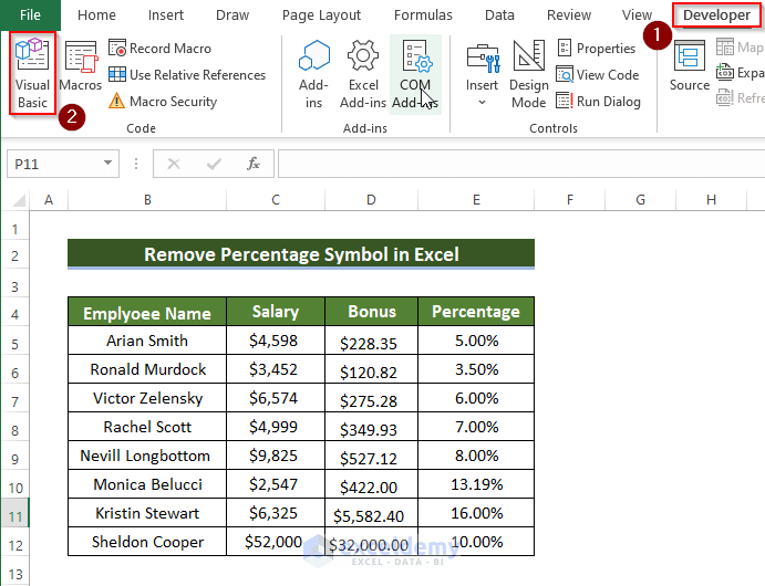
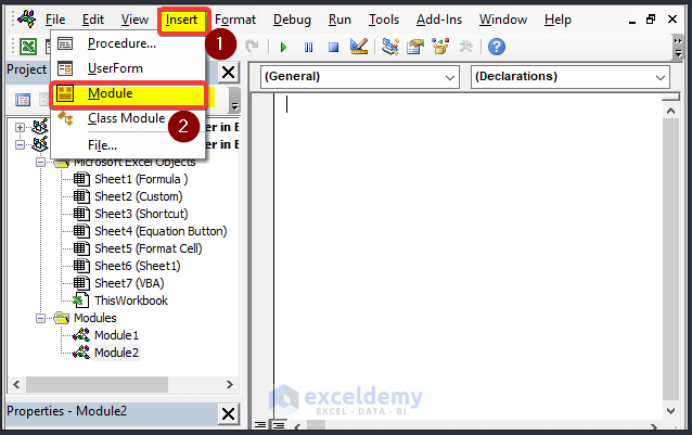
- Go to the Developer tab and click Visual Basic.
- Click Insert and select Module.
- In the Module window, enter the following code.
Sub remove_percentage_sign()

Dim rng, cell As Range
Set rng = Range("E5:E12")

For Each cell In rng

 cell.NumberFormat = "General"
 cell = cell.Value * 100

Next

End Sub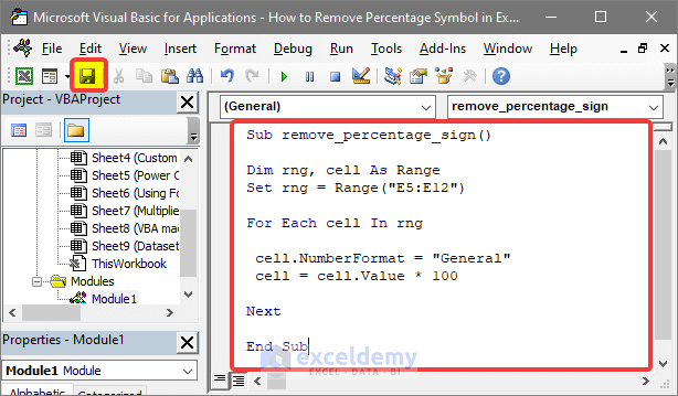
- Close the window.
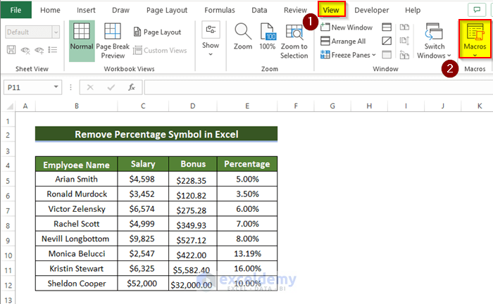
- Go to the View tab.
- Select Macros and choose View Macros.
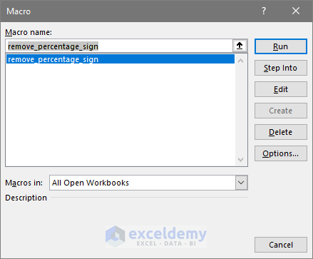
- Select the macro that you created just now. The name here is remove_percentage_sign. Click OK.
- The percentage symbol will be removed from all the numbers in the column.
Note:
In this VBA code, the range of cells E5:E12 indicates the range of input data. You need to enter a suitable range of data based on your own requirements/worksheet.
Method 6 – Utilizing the Number Formatting
Steps
- Copy the entries from the Percentage column to Percentage (Symbol Removed).
- In the Percentage (Symbol Removed) column, from the Home tab, click on text formatting in the Number group.
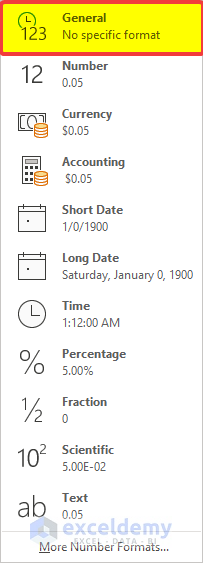
- A new menu will open. Click Number.
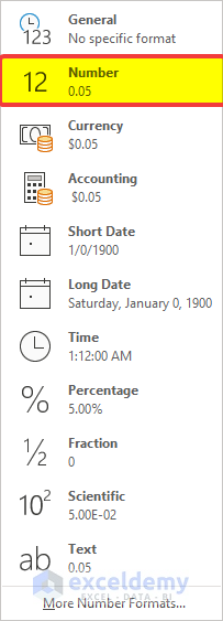
- All the numbers in the range of cells F5:F12 are now without percentages.
- The values are incorrect. Multiply all the values by 100 to get the accurate values without a percentage symbol.
Method 7 – Using General Formatting to Omit the Percentage Symbol
Steps
- Copy the entries from the Percentage column to Percentage (Symbol Removed).
- In the Percentage (Symbol Removed) column, from the Home tab, click on text formatting in the Number group.

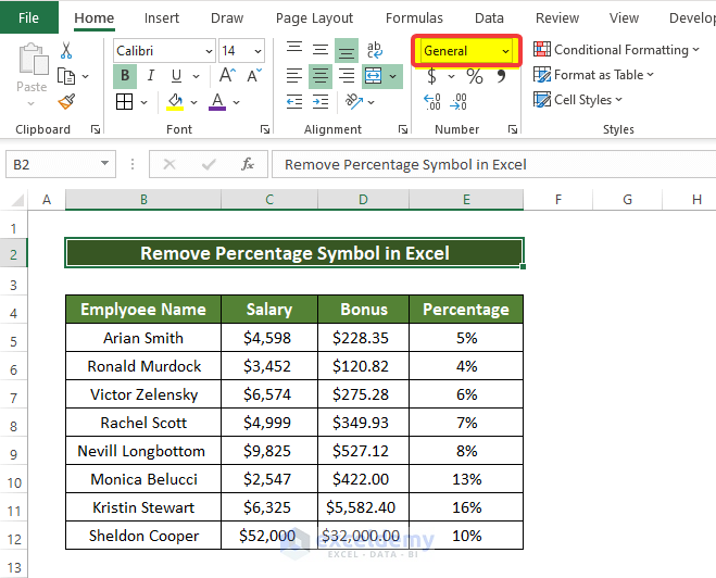
- A new menu will open. Select General.
- All the numbers in the ranges of cells F5:F12 are now without a percentage symbol.
- But their values are incorrect. Multiply the values by 100 to get the correct values.

Download the Practice Workbook
Related Articles
- How to Remove Dollar Sign in Excel
- How to Remove Dollar Sign in Excel Formula
- How to Remove Pound Sign in Excel
- How to Remove Plus Sign in Excel
- How to Remove Negative Sign in Excel
<< Go Back to Remove Symbol in Excel | Excel Symbols | Learn Excel
Get FREE Advanced Excel Exercises with Solutions!
