How to Remove Negative Sign in Excel (7 Methods)

Method 1 – Remove the Negative Sign in Excel Using the ABS Function

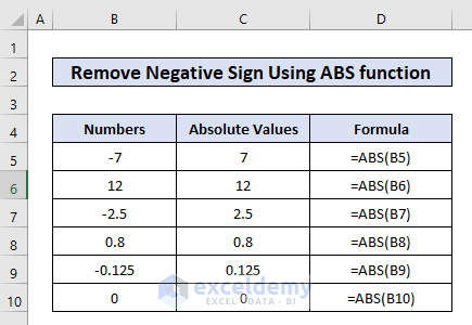
We have a list of numbers in cells B4:B10 with both positive and negative.

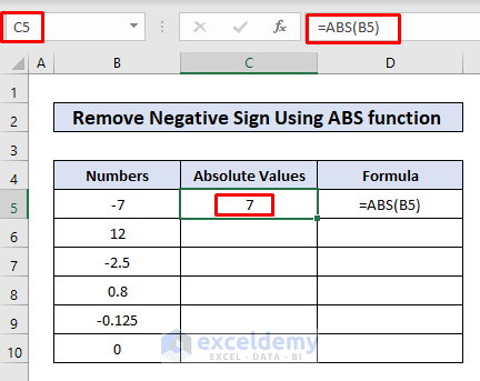
• In cell C5, enter the following formula.

Cell B5 contains a negative number -7. The result is 7 as the ABS function removes the negative sign from it.

• Use the Autofill Handle for the remaining cells.

Read More: How to Remove Plus Sign in Excel

Method 2 – Find and Replace the Negative Sign in Excel

Steps:

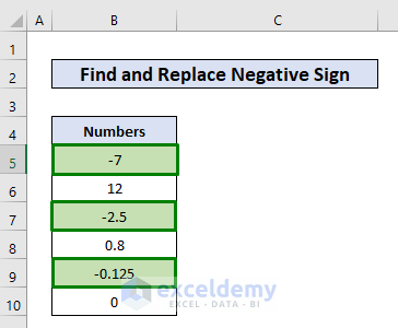
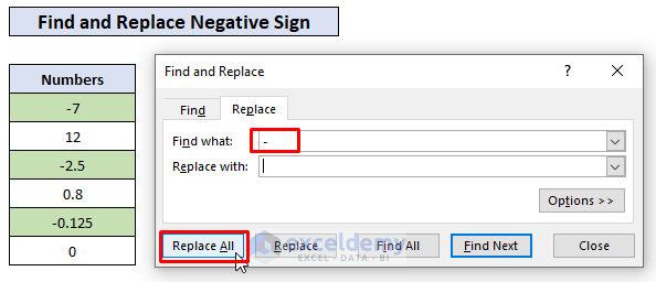
• We have three negative numbers in our dataset.

• Go to Find & Select and choose Replace.

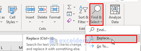
• In the Find and Replace window, put a minus (-) sign in the Find what input box and leave the Replace with input box blank.
• Click Replace All.

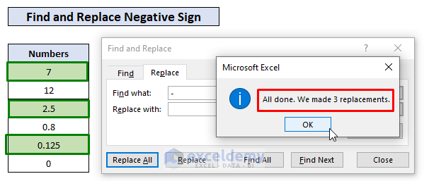
• You will receive a confirmation message. Click OK and Close.

Read More: How to Remove Sign from Numbers in Excel

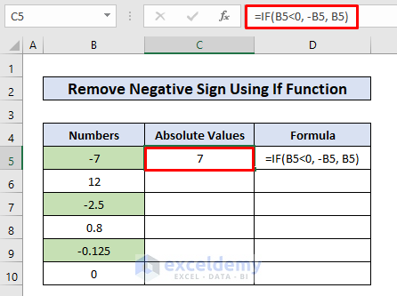
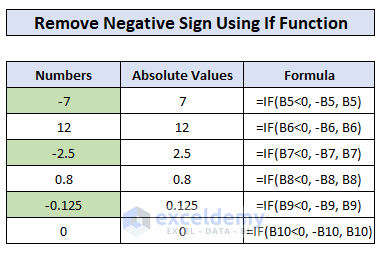
Method 3 – Use the IF Function to Check and Remove Negative Signs in Excel

• In cell C5, enter the following formula.

This will remove the negative sign from cell C5.

Copy the formula to the other cells by using the Fill Handle.

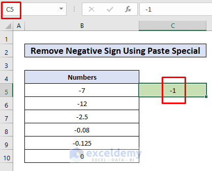
Method 4 – Reverse the Negative Sign to Positive with the Paste Special Multiplication

Steps:

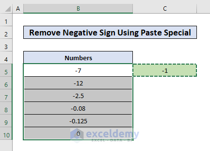
• In cell C5, enter -1 which will be used to multiply with the negative numbers in cells B5:B10.

• Copy cell C5 and select the cell range B5:B10.

• Right-click on any of the selected cells B5:B10 and click on Paste Special.

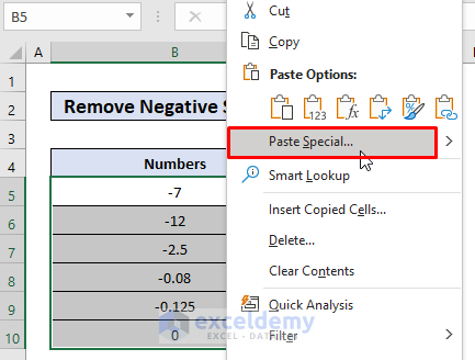
• In the Paste Special window, select Values from the Paste options and Multiply from the Operation.
• Click OK to save the changes.

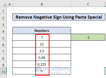
• The negative signs will be removed from the numbers.

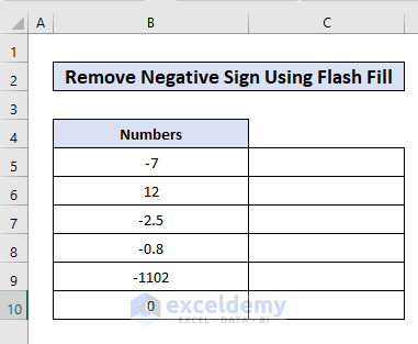
Method 5 – Remove the Negative Sign in Excel Using Flash Fill

Steps:

• We have negative numbers in cells B5:B10.

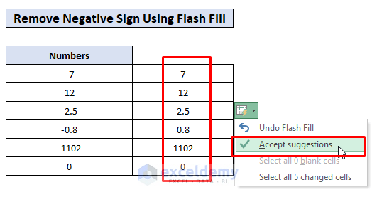
• Enter 7 in B5.

• In cell C6, press Ctrl + E.
• The above steps will flash-filled cells C6:C10 with numbers without the negative signs.
• Click on the small icon next to the flash-filled cells and click on Accept suggestions.

Method 6 – Add Custom Formatting to Remove the Negative Signs

Steps:

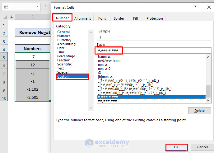
• Select cells B5:B10 that contain negative numbers.
• Press Ctrl + 1 to open the Format Cells window.
• In the Format Cells window, click the Custom option from the Category list under the Number tab.
• In the Type input box, enter #,###, #,### number format code. Press

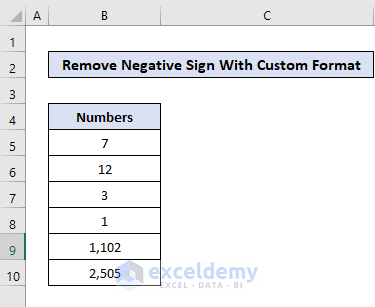
• You’ll see numbers without the negative signs.

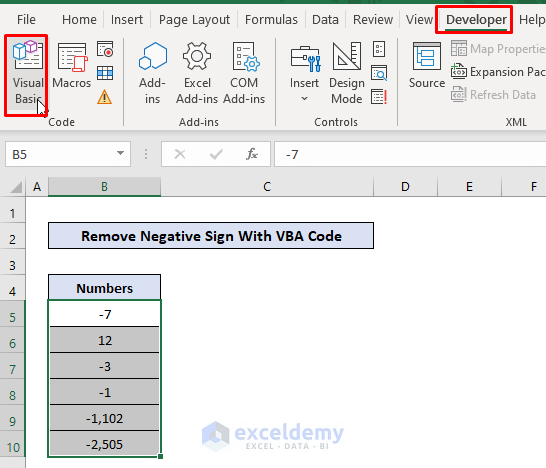
Method 7 – Apply VBA Code to Remove the Negative Sign from Selected Cells

Steps:

• Select the cells B5:B10 that contain the negative numbers.
• From the Developer tab, click on the Visual Basic option.

• Click on the Insert tab and choose Module.

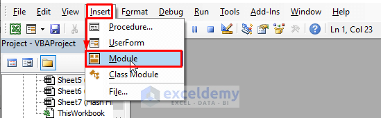
• Enter the following code and press F5 to run.

Sub RemoveNegativeSign()
For Each Cell In Selection
    If Cell.Value < 0 Then
        Cell.Value = -Cell.Value
    End If
Next Cell
End Sub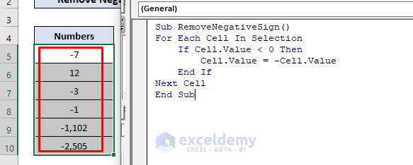

Explanation:
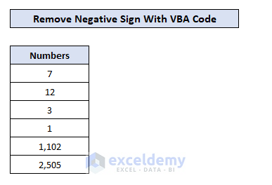
In the VBA code, the For Each loop will apply the If…Then…End If condition to each of the cells of B5:B10. It checks whether the number is less than zero. If the logic is true, it’ll replace the cell value with the negative value of itself. As a result, it’ll change it into a positive number.

Alternative Code:

Sub RemoveNegativeSign()
Dim SelectedCells As Range
For Each SelectedCells In Selection
If SelectedCells.Value <> "" Then
If IsNumeric(SelectedCells.Value) Then
SelectedCells.Value = Abs(SelectedCells.Value)
End If
End If
Next SelectedCells
End Sub

This code uses the ABS function to get only the values of the selected cells.

Download the Practice Workbook

Related Articles

• How to Remove Currency Symbol in Excel
• How to Remove Dollar Sign in Excel
• How to Remove Dollar Sign in Excel Formula
• How to Remove Pound Sign in Excel
• How to Remove Percentage Symbol in Excel
• How to Remove Percentage Symbol in Excel Without Changing Values

<< Go Back to Remove Symbol in Excel | Excel Symbols | Learn Excel