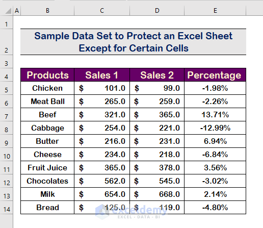
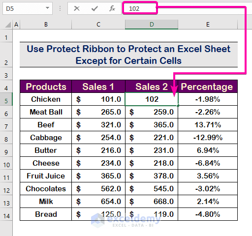
We’ll use the following sample dataset to protect the sheet except for select cells.
Method 1 – Use the Protect Ribbon to Protect an Excel Sheet Except for Certain Cells
Steps
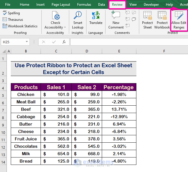
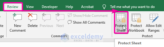
- Click on the Review tab.
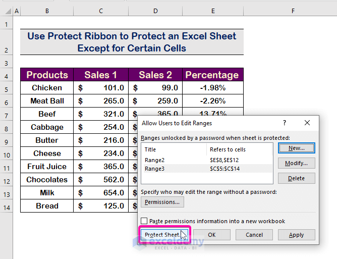
- From the Protect ribbon, select Allow Edit Ranges.
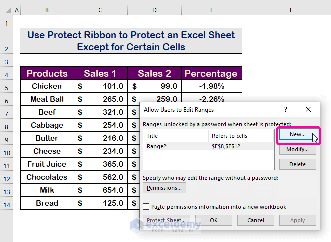
- Click on the New option.
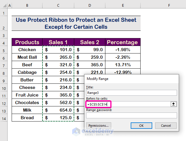
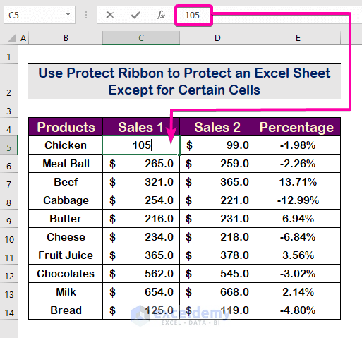
- Select the ranges (C5:C14) or cells which you want to keep unprotected.
- Press Enter.
- Click on Protect Sheet.
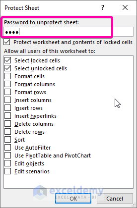
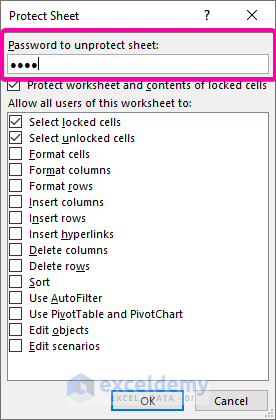
- Type any password (e. 1234) you prefer.
- Press Enter.
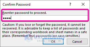
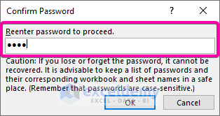
- Retype the password to confirm.
- Click OK.
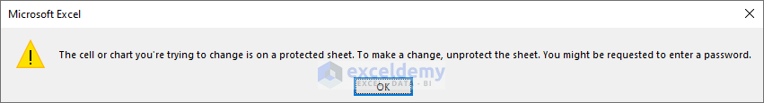
- Try to edit any cell except the range you selected.
- Excel will show the warning message that the cells are protected.
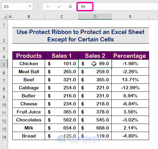
- Try to edit any cell (such as C5) from your selected range (C5:C14). You will be able to edit the cell.
Notes: To unprotect the cells, follow the steps below:
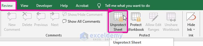
- Click on the Review tab.
- Click on Unprotect Sheet.
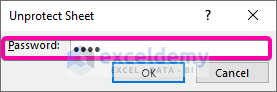
- Type in the password (e., 1234) you used to protect the sheet.
- Click OK.
- You can now edit any unprotected cells.
Read More: How to Protect Excel Sheet from Viewing Using Password
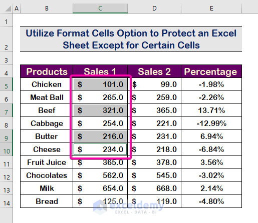
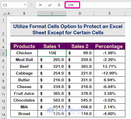
Method 2 – Utilize the Format Cells Option to Protect an Excel Sheet Except for Certain Cells
Steps:
- To select multiple cells, hold the Ctrl key and click on the cells or drag over ranges. We have selected cells C5, C7, C9, and C10.
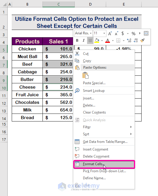
- Right-click over the selection.
- Select the Format Cells option from the list.
- In the Format Cells box, click on Protection.
- Uncheck the Locked option.
- Click OK.
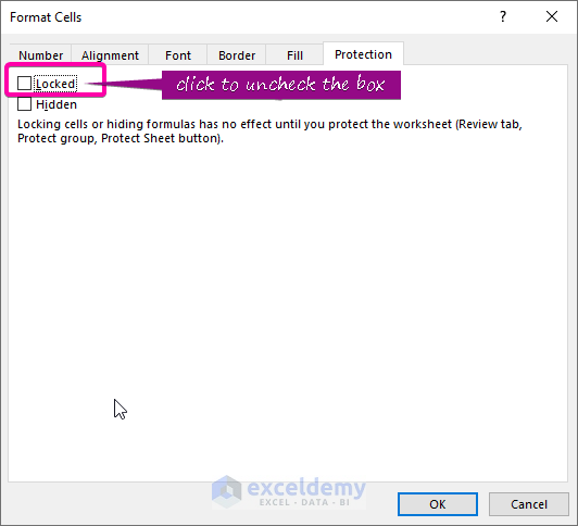
Notes: By default, in Excel Format Cells, the Locked option is enabled. Disabling the Locked option for selected cells means the selected cells will be unprotected.
- Go to the Review tab and click on the Protect Sheet command.
- Enter a password (e., 1234) you prefer.
- Press Enter.
- Retype the password.
- Click OK.
- If you attempt to change any cells that are not part of your selection, a warning message will appear informing you that the cells are protected.
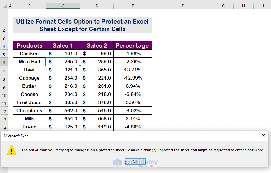
- However, you can edit the cells that were unlocked.
Read More: How to Protect Excel Sheet with Password
Download the Practice Workbook
Related Articles
- Excel VBA to Protect Sheet but Allow to Select Locked Cells
- How to Password-Protect Hidden Sheets in Excel
<< Go Back to Protect Excel Sheet | Excel Protect | Learn Excel
Get FREE Advanced Excel Exercises with Solutions!
