Download Practice Workbook
Method 1 – Moving Columns with Mouse Cursor
- Select all the cells of the column that you want to move.
- Place the cursor on the edge of the selected area and press the Shift key.
- Drag the selected column by pressing the left-click on the mouse and place it at your desired location.
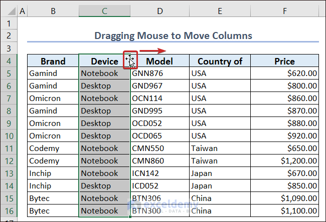
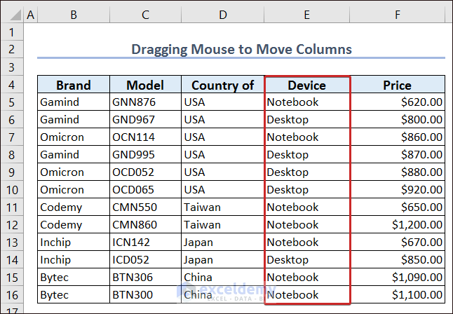
- Release the left-click and Shift button and you will have your selected column moved to the desired location.
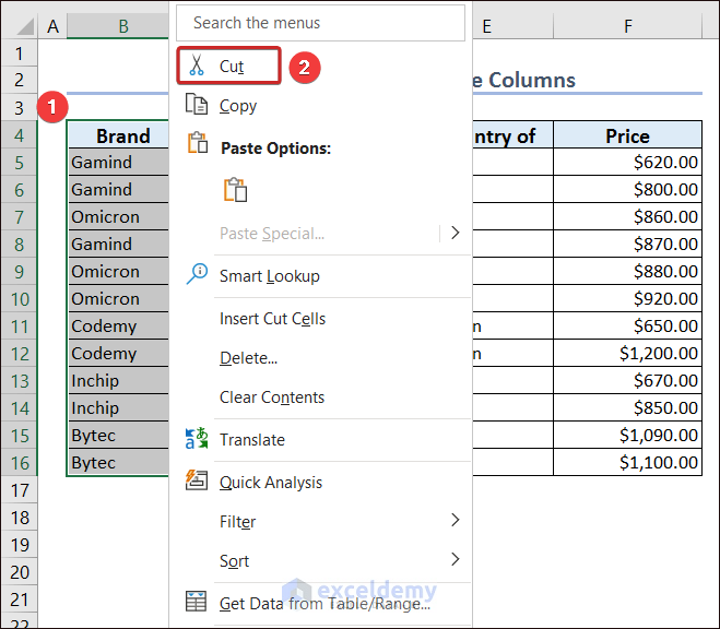
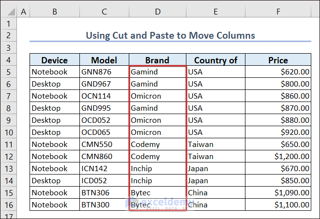
Method 2 – Use of Cut and Paste to Move Columns
- Select all the cells of a column and click on Cut after right-clicking on the mouse.
- Select a cell and right-click on the mouse. Pick the Insert Cut Cells option.
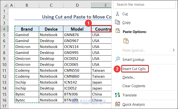
- The cut column will be pasted on the left column of the selected cell.
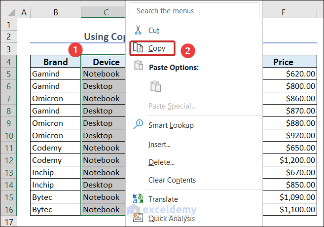
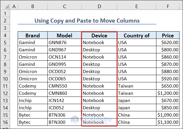
Method 3 – Moving Columns with Copy and Paste?
- Select all the cells in a column and right-click on the mouse.
- Click on Copy.
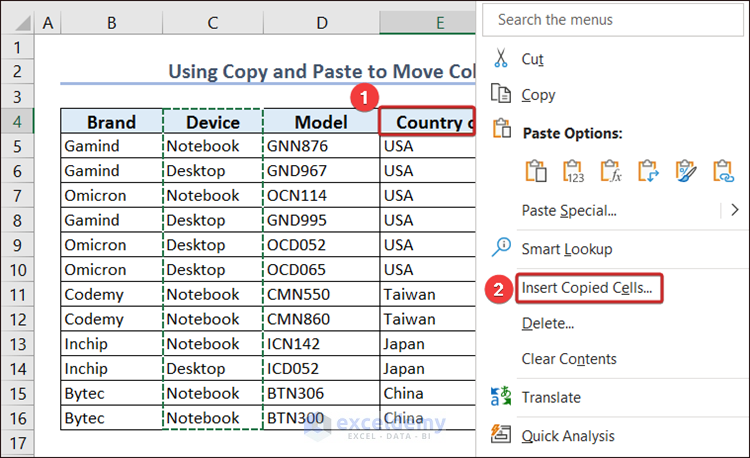
- Select a cell and right-click on the mouse.
- Click on the Insert Copied Cells…
- Select the Shift cells right option and click OK to have the copied column on the right side of the selected cell.
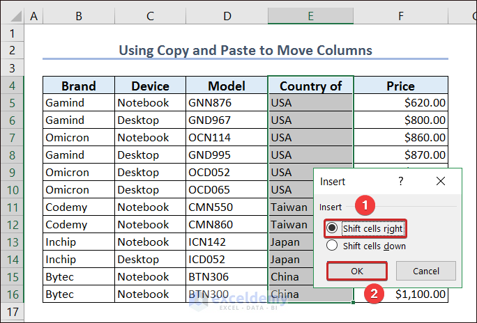
- Delete the data from the previous location and the copied column will be moved.
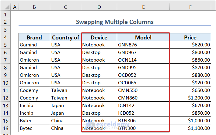
How to Swap Multiple Columns in Excel?
- Select all the cells of multiple columns and place the cursor on the edge of the selected area by pressing the Shift key.
- Drag the selected columns by pressing the left-click on the mouse and placing them at your desired location.
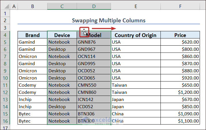
- Release the left-click and Shift button and you will have your selected columns moved to the desired location.
Read More: Move Columns in Table
Frequently Asked Questions
1. Can I undo a column move in Excel?
Yes, press Ctrl + Z to undo the column move.
2. Will the hidden columns be moved in Excel?
When selecting multiple columns for moving, if there is any hidden column in the selected area, it will be moved even if the column is hidden.
3. Is it possible to move columns containing merged cells?
No, columns containing merged cells can’t be moved.
Move Columns in Excel: Knowledge Hub
<< Go Back to Columns in Excel | Learn Excel
Get FREE Advanced Excel Exercises with Solutions!
