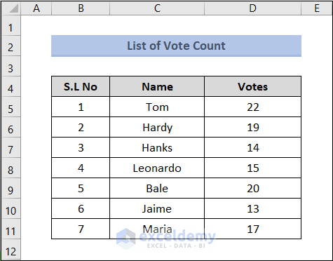
This article will use the Vote Count List dataset, which includes individual’s Names and their total Votes.
Method 1 – Using the REPT Function
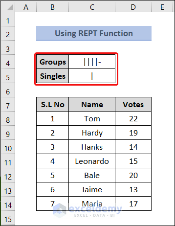
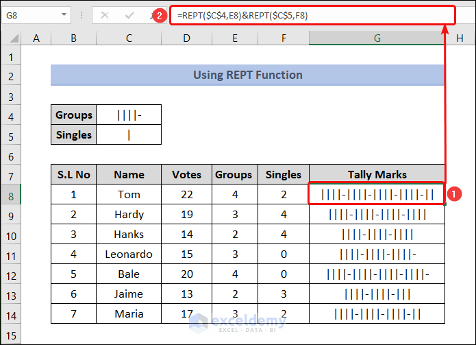
Before using the REPT function, you must define what your tally marks will look like. For four lines, you can use four vertical straight lines just above the backslash key on the keyboard. As a substitute of the diagonal strikethrough line, you can use a hyphen ( ||||- ).
Steps:
- Select cell E8.
- Copy and paste the formula below to the Formula Bar and press Enter.
=FLOOR.MATH(D8,5)/5
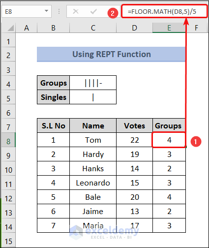
Using the FLOOR.MATH function, the value in cell D8 was rounded down to a number that is divisible by 5. Then, it was divided by 5, resulting in the quotient visible in cell E8.
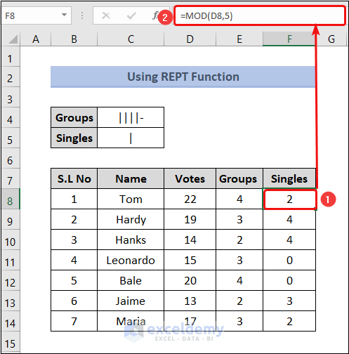
- Select cell F8, copy the formula below, and press Enter.
=MOD(D8,5)
The MOD function returns the remainder in cell F8 after dividing the value of cell D8 by 5.
- Select cell G8, copy the formula below, and press Enter.
=REPT($C$4,E8)&REPT($C$5,F8)
Cells C4 and C5 are now frozen to let the formula work properly.
Method 2 – Using a Combination of the REPT, QUOTIENT, and MOD Functions
Steps:
- Select cell E5, copy the formula below, and press Enter.
=REPT("tttt ",QUOTIENT(D5,5))&REPT("I",MOD(D5,5))
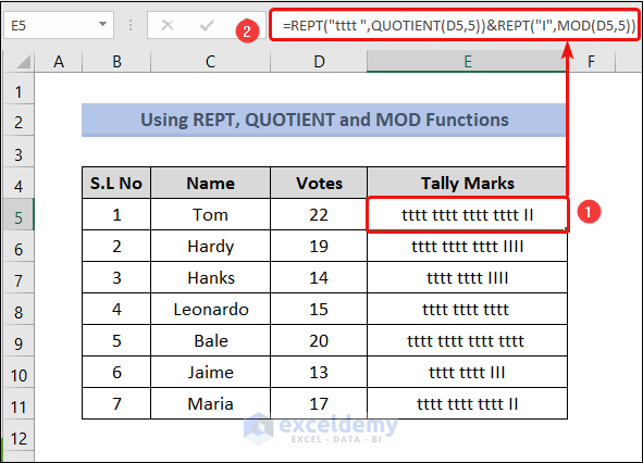
Note: While typing tttt, make sure to put a blank space at the end of the last t. Otherwise, all t’s will stick together in the E5:E11 cells.
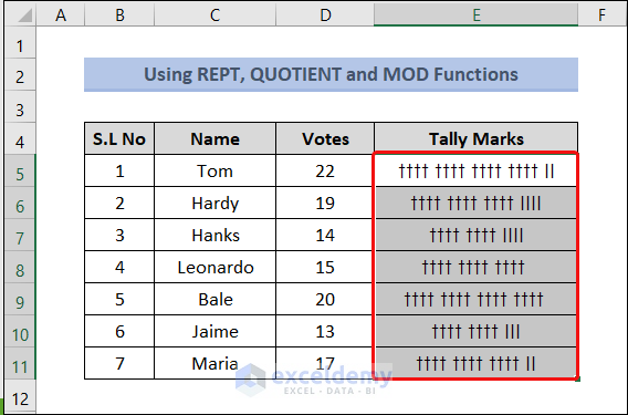
- Select the E5:E11 cell range and change the font to Century Gothic.
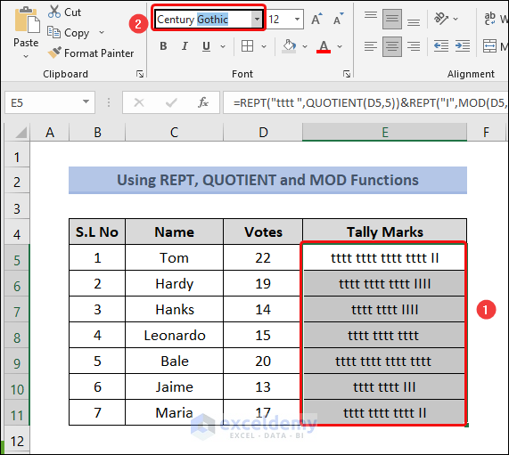
- You should be able to see the output in the correct format.
Method 3 – Creating Tally Marks From a Bar Chart
Steps:
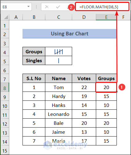
- Fill out the Groups column. For this, select cell E8, copy the formula below, and press Enter.
=FLOOR.MATH(D8,5)
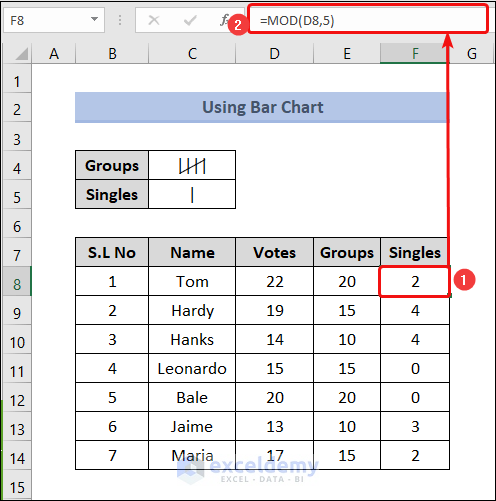
- Select cell F8, copy the formula below, and press Enter.
=MOD(D8,5)
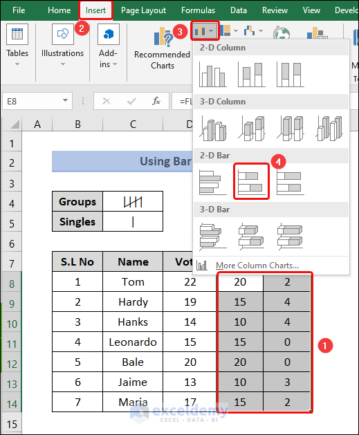
- Select cells E8:F14 and go to the Insert tab.
- Choose the Insert Column or Bar Chart option and select 2-D Stacked Bar.
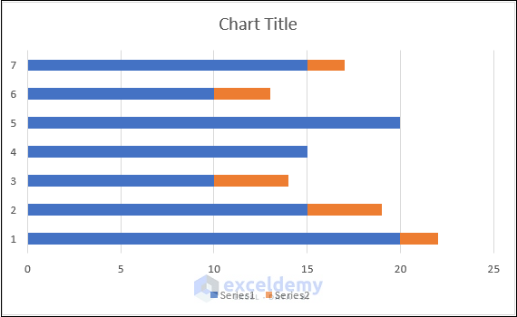
- A horizontal bar chart will appear.
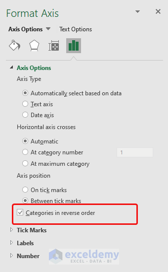
- Right-click on the y-axis and select Format Axis from the options.
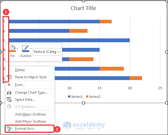
- In the Format Axis menu, check the Categories in reverse order box.
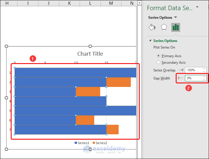
- Double-click on any bar to open the Format Data Series.
- Decrease the Gap Width to 0% to remove the gap between two bars.
- Delete the unnecessary visual elements like Chart Title, Legend, and Axis to make the graph area neater.

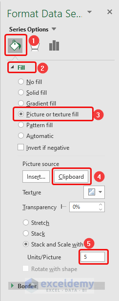
- Copy cell C4 to your clipboard and double-click on any blue bar in the graph to reopen the Format Data Series menu.
- From the Format Data Series option, select Fill and Line.
- Go to the Fill section and check the Picture to texture fill box.
- Press the Clipboard button.
- Check the Stack and Scale with box.
- Write 5 in the Unit/Picture box.
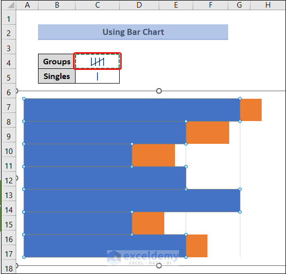
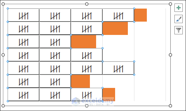
- As an example, our chart will look like this:
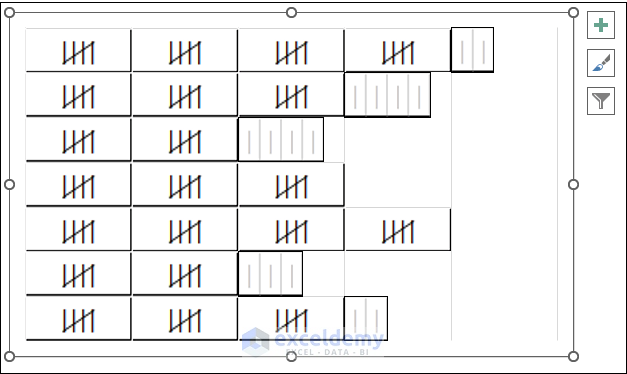
- Select cell C5, double-click on the orange-colored bar, and repeat the previous steps.
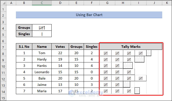
- Size down the chart to fit the table and place it next to the existing table, as pictured below.
Read More: How to Make a Tally Chart in Excel
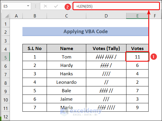
Method 4 – Applying a VBA Code to Make Tally Marks in Excel
Steps:
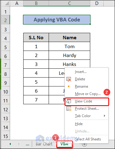
- Right-click on the Sheet name and select View Code.
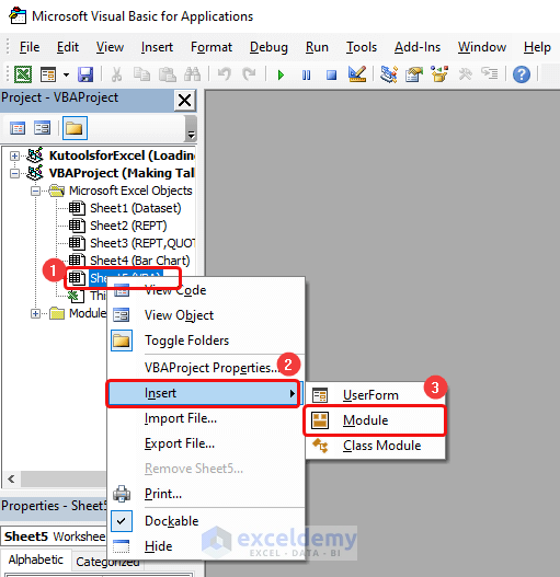
- Go to Toggle Folders and right-click on Sheet5 (VBA).
- Select the Insert option and click on Module.
- Copy and paste the following code to the code module and hit Run or press F5:
Private Sub Worksheet_BeforeDoubleClick(ByVal Target As Range, Cancel As Boolean)
Dim cells As Range
Dim i As Long, j As Long, n As Long
'Select the Range you want to apply this code to
Set cells = Me.Range("D5:D11")
Set cells = Intersect(cells, Target)
If Not cells Is Nothing Then
    Cancel = True
    Application.EnableEvents = False
    n = Len(cells.Value)
    j = n Mod 5
    If j = 4 Then
        cells.Value = cells.Value & " "
    Else
    'Select the tally sign you want for each doubleclick
        cells.Value = cells.Value & "/"
    End If
         cells.Font.Strikethrough = False
    For i = 1 To n Step 5
        If (j = 4) Or (i < (n - j)) Then
            cells.Characters(i, 4).Font.Strikethrough = True
        End If
    Next
    Application.EnableEvents = True
End If
End Sub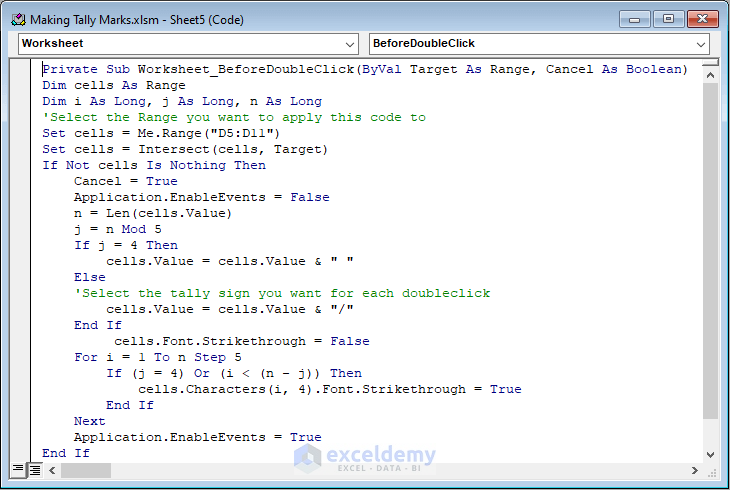
- Close the code module and return to the worksheet.
- Double-click on any cell in column D to put a tally mark in the cell.
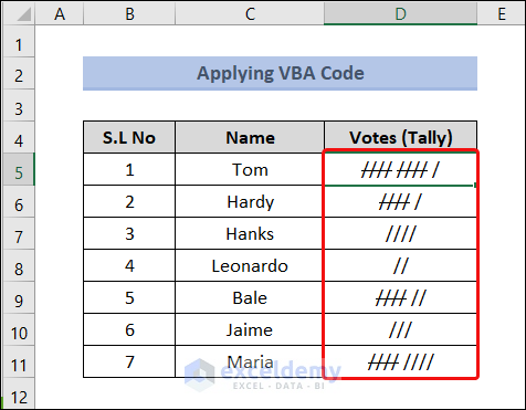
- Select cell E5, copy the formula below, and press Enter to count the tally and display it in number format:
=LEN(D5)
Read More: How to Make a Tally Sheet in Excel
Download Practice Workbook
Feel free to download the following Excel workbook for better understanding and self-practice.
Related Articles
- How to Create a Tally Button in Excel
- How to Tally Words in Excel
- How to Tally a Column in Excel
- How to Tally Votes in Excel
- How to Export Tally Data in Excel
<< Go Back to Tally in Excel | Excel for Statistics | Learn Excel
Get FREE Advanced Excel Exercises with Solutions!
