How to Make Legend Markers Bigger in Excel (3 Easy Ways)

In this article, we will learn to make legend markers bigger in Excel. Legend markers are used to denote the data with specific colors. Sometimes, legend markers become small to see after plotting the chart. In that case, we need to make the legend markers bigger. Today, we will demonstrate 3 easy methods. Using these methods, you can easily make legend markers bigger in Excel. So, without any delay, let’s start the discussion.

How to Make Legend Markers Bigger in Excel: 3 Easy Ways

To explain these methods, we will use a dataset that contains information about the sales amount of some sellers for the first two months. We will plot the dataset graphically and make the legend markers bigger.

After plotting the graph on a Clustered Column chart, you will see results like the picture below. You can see the legend markers are smaller. We will make these markers bigger using the following methods.

1. Change Font Size to Make Legend Markers Bigger in Excel

The easiest way to make legend markers bigger in Excel is to change the font size of the legend. It will increase the size of the marker as well as the font size. Let’s follow the steps below to see how we can change the font size.

STEPS:

• First of all, right–click on the Legend Box to open the Context Menu.
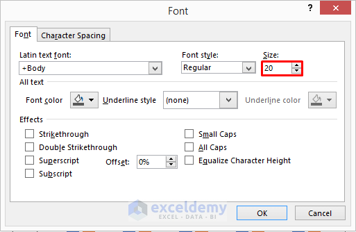
• Select Font from there. It will open the Font dialog box.

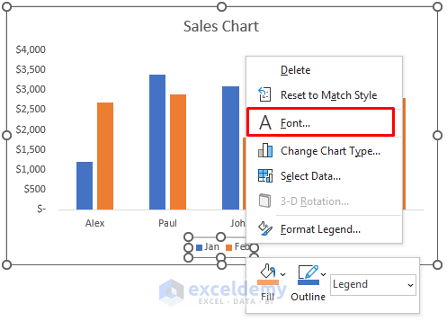
• Secondly, set the font size to 20 in the Font dialog box. You can change it according to your preference.
• Click OK to proceed.

• As a result, you will see bigger legend markers on the chart.

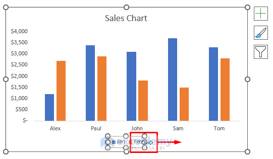
• Also, you can increase the chart area using the double–headed arrow.

• Finally, the legend markers will look more significant than in the previous scenario.

Read More: How to Add Data Markers in Excel 

2. Make Bigger Legend Markers by Adding Dummy Series

Another effective way to make bigger legend markers is to add dummy series in the dataset. This process is effective because it increases the size of the markers only. It doesn’t make the font size bigger. In this method, we will use the same dataset. But we need to add a helper column.

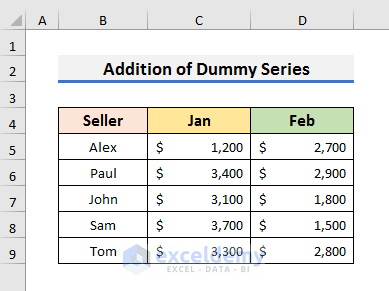
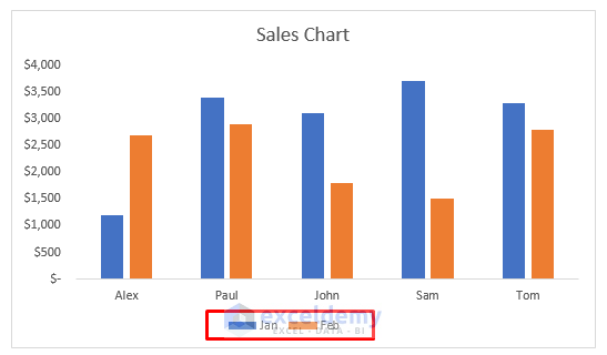
After plotting the chart, you can see two legends with small markers.

Let’s follow the steps below to see how we can make bigger legend markers using dummy series.

STEPS:

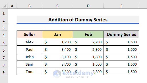
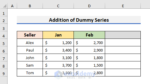
• Firstly, fill the Dummy Series column with a constant value.

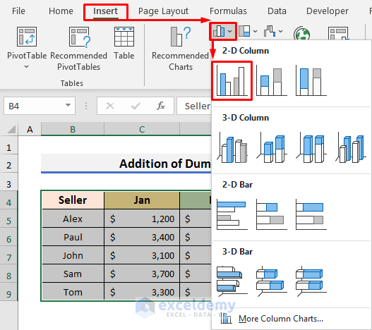
• Secondly, select all cells of your dataset and then, go to the Insert tab.
• Select the Insert Column icon and then, select Clustered Column from the drop-down menu.

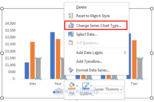
• As a result, you will see the data of the Dummy Series on the chart. Here, the gray columns are denoting the Dummy Series.
• You can also see the legend of the Dummy Series in the legend box.

• Now, right–click on the gray column and select Change Series Chart Type from the menu. It will open the Change Chart Type dialog box.

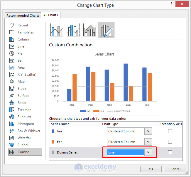
• In the Change Chart Type window, change the Chart Type of the Dummy Series to Line.
• Click OK to proceed.

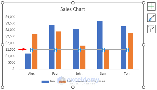
• As a result, you will see a straight line on the chart.
• Double–click on the straight line to open the Format Data Series settings.

• In the Format Data Series settings, click on the Fill icon.
• Select the Solid line option from there and set the color to White.

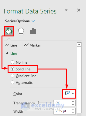
• After that, the gray straight line will change into a white line.
• Also, the Legend Marker of the Dummy Series will vanish.

• At this moment, remove the contents from the Dummy Series.

• Finally, the legend markers will be bigger on the chart and it will contain no information about the Dummy Series.

Read More: How to Add Markers for Each Month in Excel 

3. Increase Legend Markers Size Using Format Tab in Excel

In the last method, we will use the Format tab to increase the size of the legend markers. We add shapes to the chart and place them on top of the markers.  In this way, we can make the legend markers look bigger. Here, we will use the same chart. So, without further ado, let’s follow the steps below.

STEPS:

• In the beginning, we need to increase the size of the legend box.
• To do so, click on the legend box and move the double–headed arrow to the right.

• After increasing the legend box size, the legends will be placed far from each other.

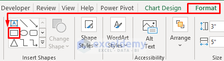
• In the following step, select the chart and then, navigate to the Format tab in the ribbon.
• Select Rectangular shape from the Insert Shapes You can select other types of shapes according to your legends.

• After selecting the shape, the mouse pointer will change into a small black plus (+) sign.
• Using the small black plus (+) sign, you need to draw the shape and place it on top of the first legend like in the picture below.

• After that, select the shape and press Ctrl + C to copy it.

• Now, press Ctrl + V to paste it on the chart and place it on the second legend.

• At this moment, you need to change the color of the second legend.
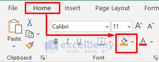
• For that purpose, select the second legend and go to the Home tab.
• Use the Fill Color option to fill the second legend with the appropriate color.

• Finally, you will be able to make legend markers bigger in Excel.

Read More: How to Change Marker Shape in Excel Graph

Download Practice Book

You can download the practice book from here.

Conclusion

In this article, we have discussed 3 easy methods to Make Legend Markers Bigger in Excel. I hope this article will help you to perform your tasks easily. Furthermore, we have also added the practice book at the beginning of the article. To test your skills, you can download it to exercise. Last of all, if you have any suggestions or queries, feel free to ask in the comment section below.

<< Go Back To Markers in Excel | Excel Charts | Learn Excel