How to Change Marker Shape in Excel Graph (3 Easy Methods)

Excel automatically creates a shape for the marker when creating a Line, (XY) Scatter, and Radar chart. These data markers help to visualize the value of the data point clearly. However, in many situations, we need to change marker shapes so that they become more visible and eye-catching.

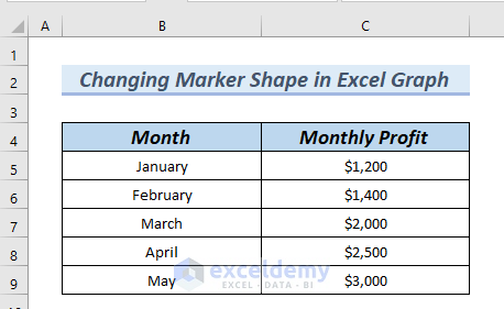
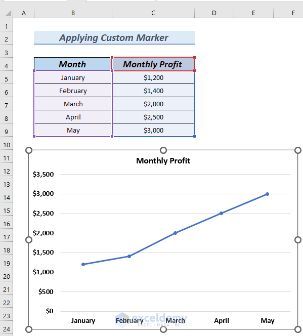
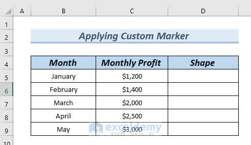
The following dataset has Month and Monthly Profit columns.

Using this dataset we will insert a Line with Markers chart, then change the marker shapes. We used Excel 365 here, but you can use any available Excel version.

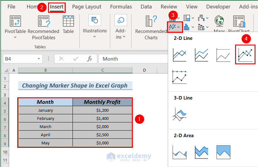
To insert a Line with Markers chart:

Select the entire dataset.
Go to the Insert tab.
From Insert Line or Area Chart group, select the Line with Markers chart.

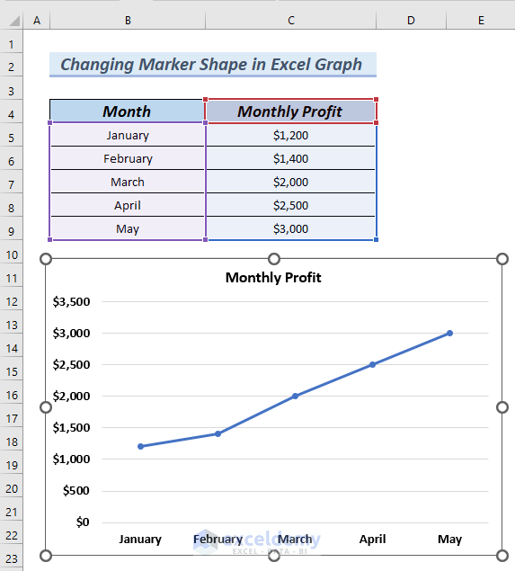
A Line with Markers chart is generated, with clearly visible marker points on it.

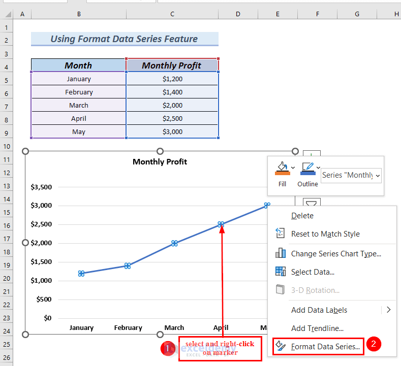
Method 1 – Using Format Data Series Feature

STEPS:

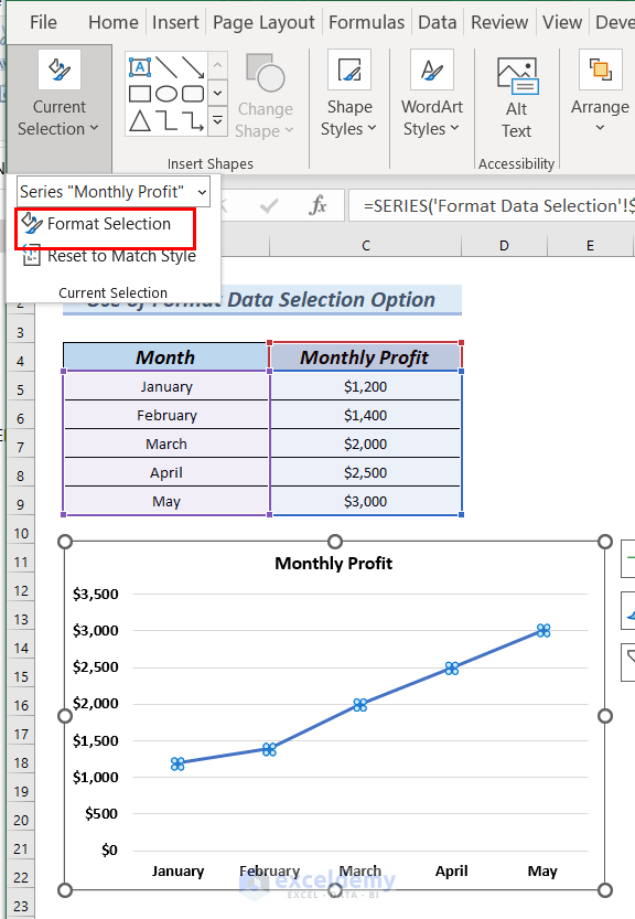
Click on any marker of the graph, which will automatically select all the markers of the graph.
Right-click on it.
Select Format Data Series from the Context Menu.

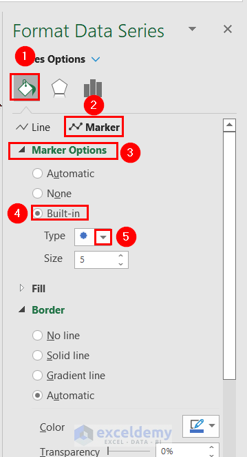
A Format Data Series dialog box will appear at the right end of the Excel sheet.

Select the Fill & Line option >> select Marker >> select Marker Options.
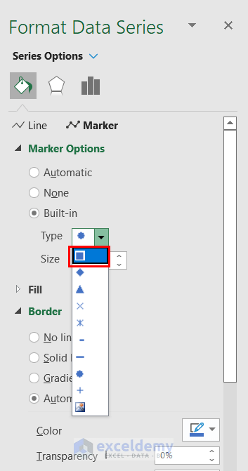
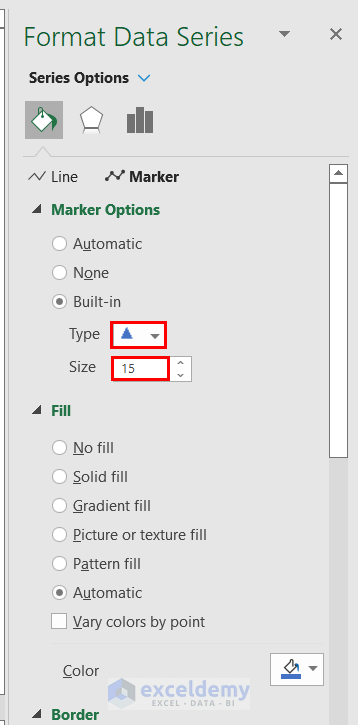
From Marker Options >> select Built-in box.
Click on the downward arrow of the Type box.

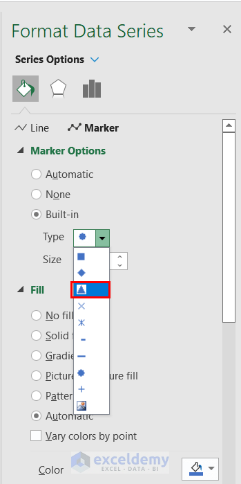
Several marker shapes appear. Select any of them according to your preference.

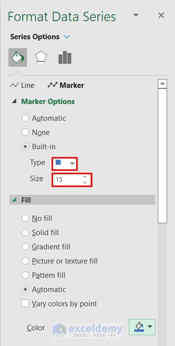
Select a rectangle as a marker shape.

In the Type box, a rectangular shape appears.

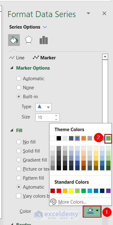
Set the Size to 15 (you can select any Size of your choice).

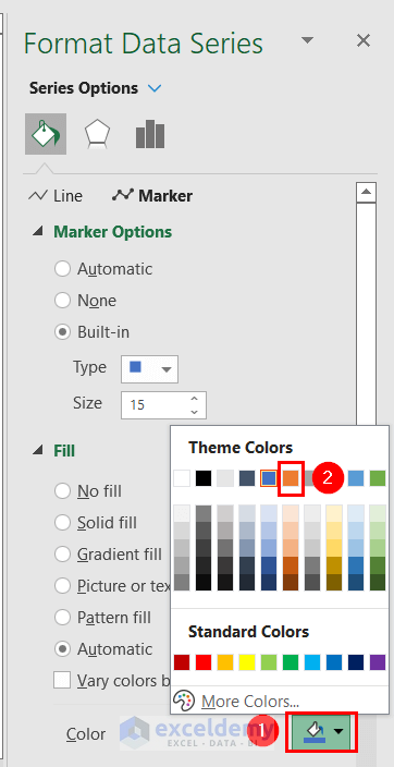
Click on the drop-down arrow of the Color box.
Select Orange, with Accent 2 as our marker color.

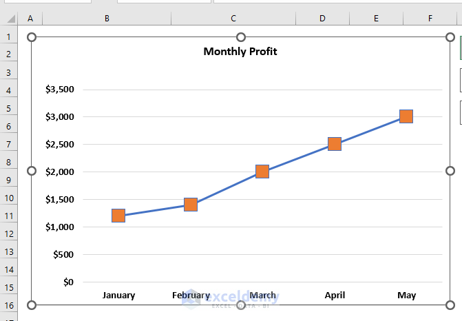
The graph now has rectangular marker shapes.

Read More: How to Add Data Markers in Excel

Method 2 – Using Format Selection Option

STEPS:

Click on any marker of the graph, which will automatically select all the markers of the graph.
Go to the Format tab >> click on Current Selection.

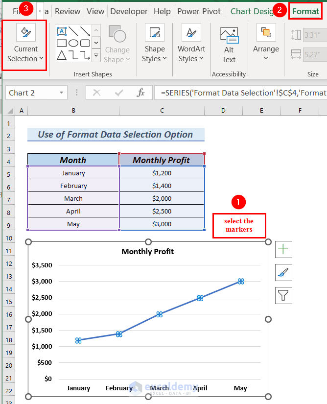
From the Current Selection group, select the Format Selection option.

A Format Data Series dialog box appears at the right end of the Excel sheet.

Select the Fill & Line option >> select Marker >> select Marker Options.
From Marker Options >> select Built-in box.
Click on the downward arrow of the Type box.

Several marker shapes appear. You can select any marker shape of your choice.

Select a triangle as a marker shape.

In the Type box, a triangular shape is shown.

Set the Size to 15 (or any Size of your choice).

Click on the drop-down arrow of the Color box.
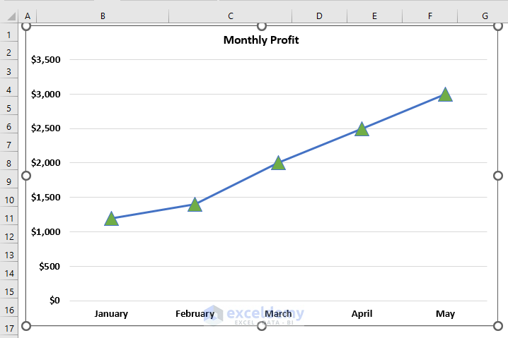
Select Green, Accent 6 as our marker color.

The graph now has triangular marker shapes.

Method 3 – Using a Custom Marker

You can change the marker shape in an Excel graph by inserting custom pictures or shapes for individual marker points.

STEPS:

Create a Shape column in our dataset.

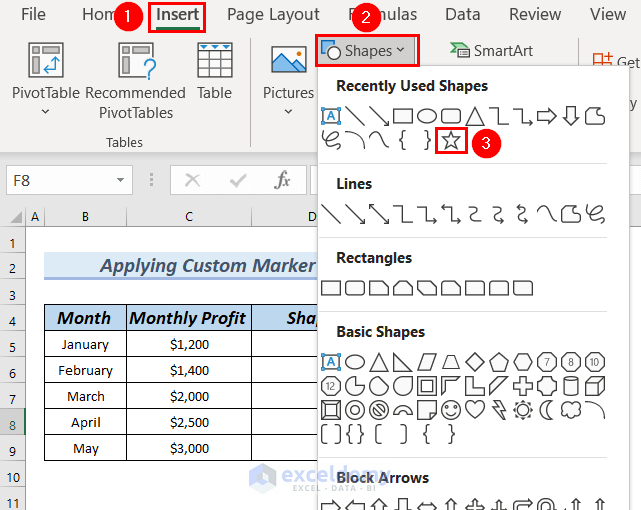
Go to the Insert tab >> click on Shapes.

A huge number of shapes is displayed.

Select the Star shape.

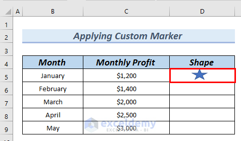
Insert the Star shape in cell D5 for January month.

Now we insert this shape in the graph.

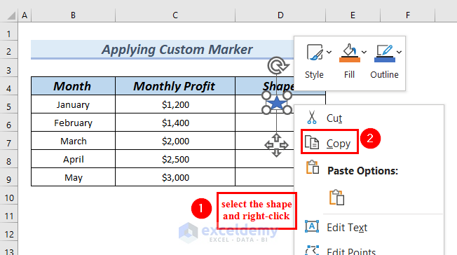
Select the Star shape and right-click on it.
Select the Copy option from the Context Menu.

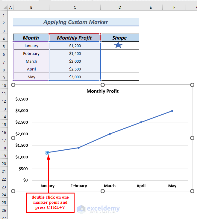
On our chart, double click on the January marker (a double-click will select one single marker point).

Press CTRL+V to paste the copied Star shape on the marker.

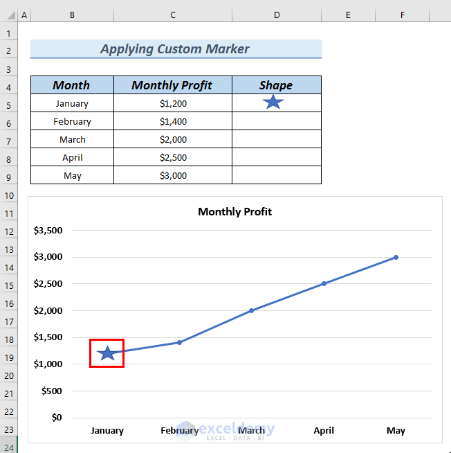
The marker for January month now has a Star shape.

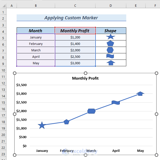
Repeat the same process to insert different shapes for every individual month in the Shape column.
Copy the shapes and paste them onto the markers of the graph.

The markers on the graph now have different shapes.