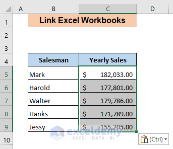
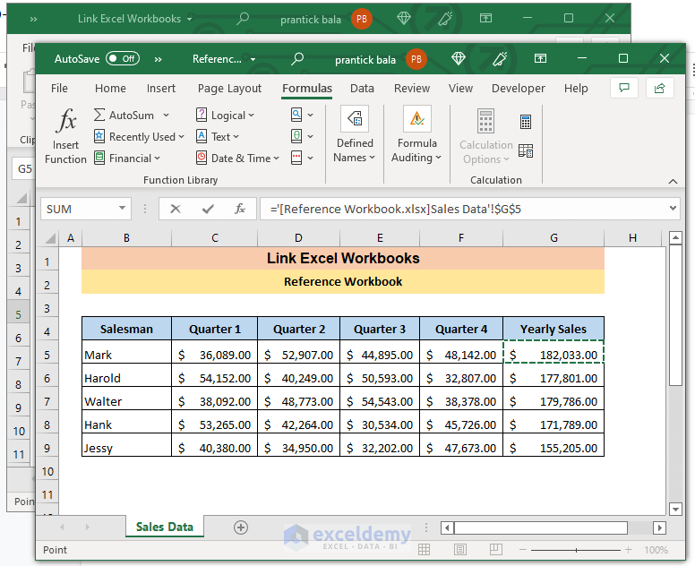
You have sales data of different salesmen in the “Sales Data” sheet of the “Reference Workbook” workbook.
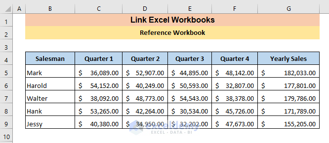
To extract “Yearly Sales” from the Reference Workbook to a sheet named “Sales Summary” in the “Link Excel Workbooks” workbook:
Method 1 – Link Excel Workbooks Using the Paste Link Option
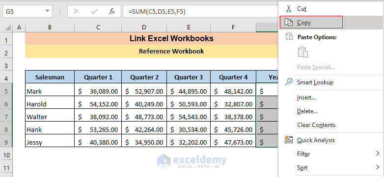
- Select the cells in the “Yearly Sales” column (“Reference Workbook”) and right-click.
- In the context menu, click Copy.
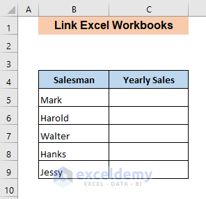
- Open “Link Excel Workbooks”.
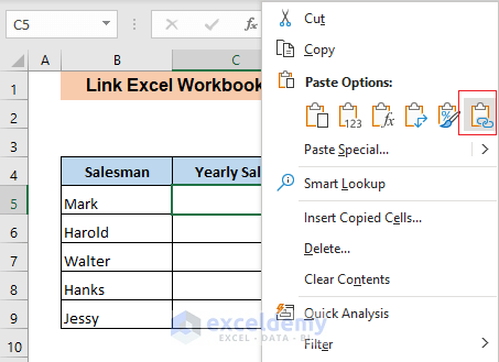
- Right-click C5 (first cell of “Yearly Sales” column)
- In the context menu, click Paste Link in Paste Options.
The “Reference Workbook” will be linked to the current workbook.
If you click any of the linked cells, you can see it refers to another workbook in the formula bar.
Method 2 – Switching Between Two Workbooks
- Open both workbooks.
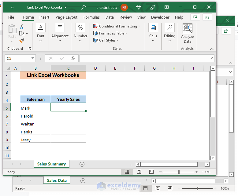
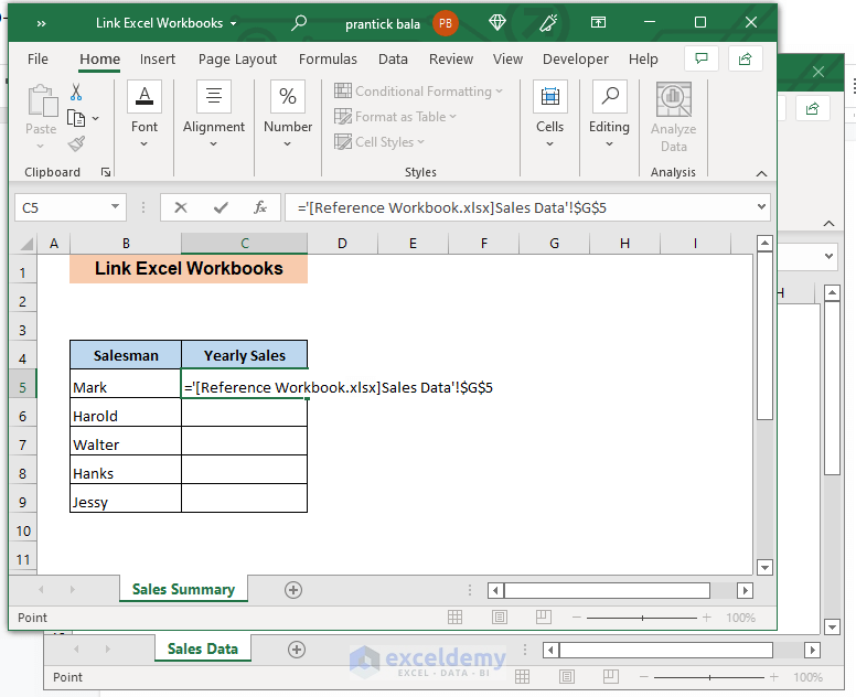
- Enter = in C5 (first cell of the “Yearly Sales” column).
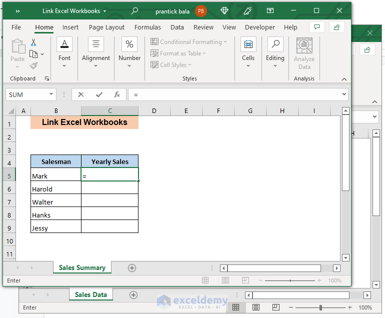
- Go to the “Reference Workbook” and click G5 (first cell of “Yearly Sales” column in the “Reference Workbook”)
- Go back to the first workbook.
The selected cell of the first workbook (“Link Excel Workbooks”) refers to a cell of the second workbook (“Reference Workbook”).
- Press ENTER.
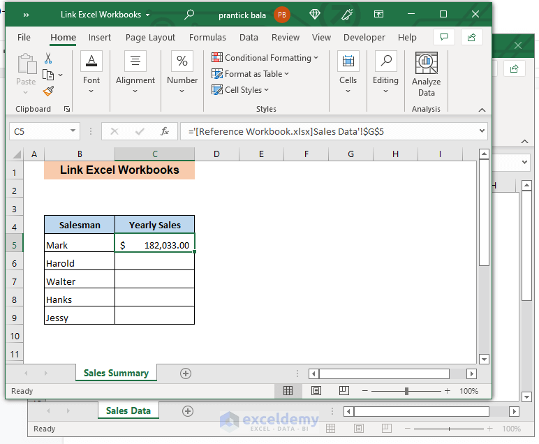
C5 will be linked to G5 of the other workbook.
Excel automatically applies Absolute reference. You need to convert this absolute reference into a relative reference.
- Delete the dollar sign ($) in the formula.
- Press ENTER.
- Drag down the Fill Handle to see the result in the rest of the cells.
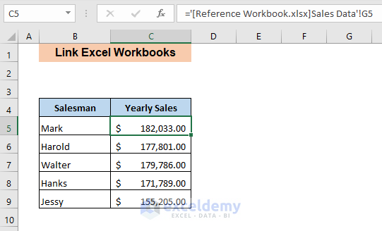
Method 3 – Entering a Formula Manually
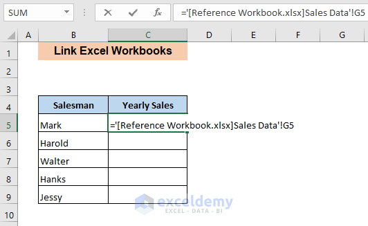
- Enter the following formula in C5,
='[Reference Workbook.xlsx]Sales Data'!G5Reference Workbook.xlsx refers to the second workbook and Sales Data refers to the datasheet containing data that will be linked to that workbook. G5 is the first cell of the “Yearly Sales” column in the Sales Data sheet of the second workbook.
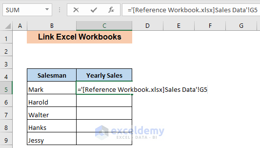
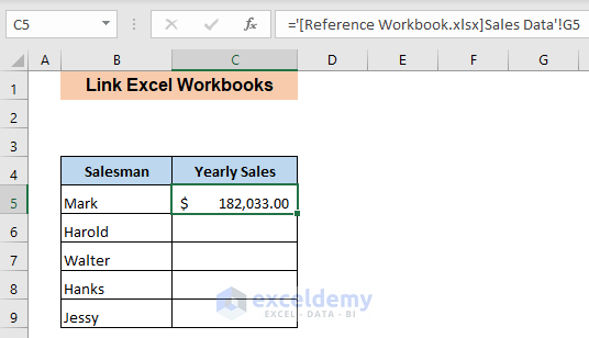
- Press ENTER.
C5 will be linked to G5 of the other workbook.
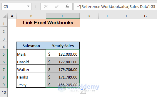
- Drag down the Fill Handle to see the result in the rest of the cells.
The “Reference Workbook” will be linked to the “Link Excel Workbooks” .
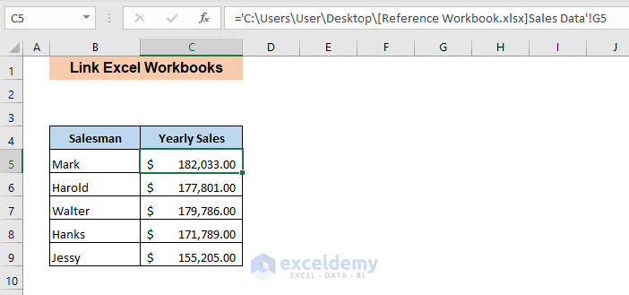
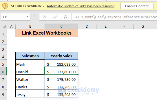
If you close the second workbook, the formula in the first workbook will automatically change:
='C:\Users\User\Desktop\Reference Workbook.xlsx]Sales Data'!G5Here, C:\Users\User\Desktop is the location of the linked workbook.
Method 4 – Linking Excel Workbooks Using a Named Range
- Open the “Reference Workbook” and select the cells in the Yearly Sales column
- Go to Formulas > Defined Names > Define Name.
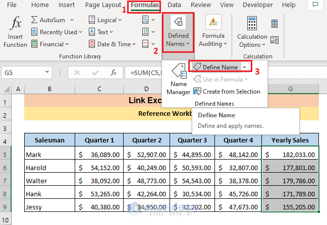
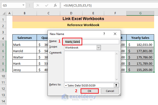
- In New Name, enter a name for the selected cells in Name.
- Click OK.
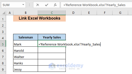
- Open “Link Excel Workbooks” and enter the following formula in C5:
='Reference Workbook.xlsx'!Yearly_SalesThe formula will link the named range to this workbook.
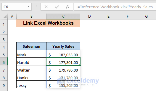
If you use Excel 365:
- Press ENTER.
If you use any other version, press CTRL+SHIFT+ENTER for the array formula.
Workbooks will be linked.
Things to Remember
When you close the workbook, Excel disables all links used. You have to enable them by clicking Enable Content in the SECURITY WARNING dialog box, after reopening the workbook.
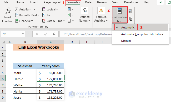
Check if the Automatic option is checked in Formulas > Calculation Options > Automatic. Otherwise, the linked cells of your workbook won’t change automatically.
Download Practice Workbooks
Linking Workbooks in Excel: Knowledge Hub
- Link Two Workbooks in Excel
- Reference from Another Excel Workbook Without Opening
- Link Excel Workbooks for Automatic Update
- [Fixed!] Excel Links Not Working Unless Source Workbook Is Open
- [Fixed!] This Workbook Contains Links to One or More External Sources That Could Be Unsafe
- [Fixed!] ‘This workbook contains links to other data sources’ Error in Excel
<< Go Back To Linking in Excel | Learn Excel
Get FREE Advanced Excel Exercises with Solutions!
