In this tutorial, I am going to show you 5 practical examples of how to calculate annuity in Excel. Finding out the various aspects of an annuity is a fairly simple task if you know the annuity’s interest rate, total amount, and duration period. However, it is important to mention that calculating this value is only feasible when you are dealing with fixed annuities.
What is Annuity?
An annuity is a contract between two parties where one party invests some amount at the start and will get an annual payment for a certain period of time from the other party. There are many variations of the annuity calculator formula. One basic type is as follows:
P = C * [(1 – (1 + r)^-n) / r]
Where,
P= Present value of the annuity
C= Future cash flow stream
r= Interest rate and
n= Number of periods which can be months or years.
How to Calculate Annuity in Excel: 5 Practical Examples
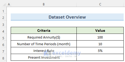
In the following examples, we will be mainly working with 4 parameters to calculate annuity in Excel. These are periodic annuity, number of periods, interest rate, and present or future value of total money. The monetary values are inserted in dollars. Also, we have taken months as unit time periods. For the interest rate, we have used the percentage format which you can find in the Number section under the tab Home.
1. Calculating Annuity Using PV Function
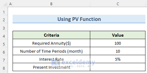
The PV function in Excel is a financial function that can calculate the present value of an investment. In this method, we will try to calculate the present amount that we need to deposit to get a fixed annuity in Excel for the next 10 months.
Steps:
- First, enter the required data as shown in the image below.
- Next, double-click on cell C8 and enter the following formula:
=PV(C7,C6,C5)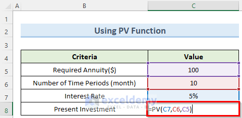
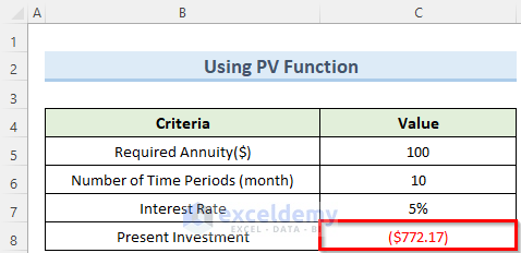
- Then, press Enter.
- As a result, you will get the amount of investment needed at present for the required future annuity.
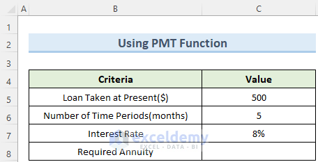
2. Applying PMT Function
The PMT function in Excel returns the periodic payment or annuity for a current loan. For this, we need to know a few parameters like time periods, interest rate, etc to calculate annuity in Excel using this function. Let us see how we can do this.
Steps:
- To begin with, enter the Loan Amount in cell C5.
- Similarly, enter the time period and the interest rate in cells C6 and C7 respectively.
- Now, click on cell C8 and type in the following formula:
=PMT(C7,C6,C5)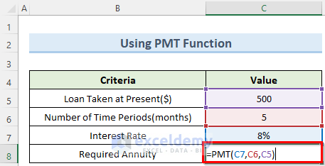
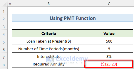
- Then, press the Enter key, and Excel will calculate the required annuity in dollars.
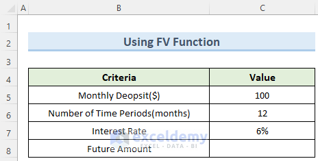
3. Using FV Function
If we want to calculate the future value of an investment then the FV function in Excel can help. This function assumes constant annuity in Excel and constant interest rates. Follow the steps below to use this function.
Steps:
- First of all, enter the monthly deposit amount in dollars in cell C5.
- Then, type in the time periods and interest rates in cells C6 and C7.
- Next, double-click on cell C8 and enter the following formula:
=FV(C7,C6,C5)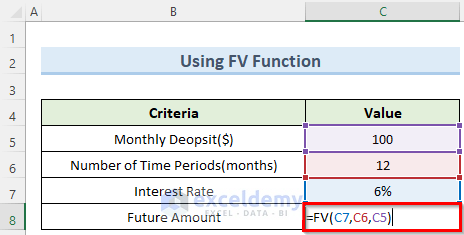
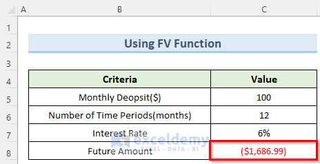
- Then, press Enter or click on any empty cell.
- Consequently, you will get the future amount that will accumulate according to the annuity.
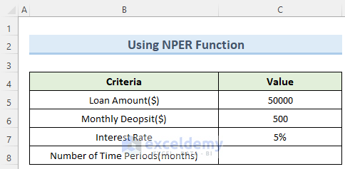
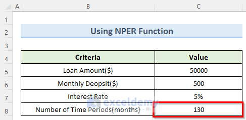
4. Finding Annuity Period Using NPER Function
The NPER function is one of the most used Excel financial functions. The function can calculate the time period required to pay off a loan at a fixed annuity.
Steps:
- To begin this method, insert suitable data in the proper cells as shown in the following image.
- Now, click on cell C8 and insert the following formula.
=NPER(C7/12,C6,-C5)- Note that, we have a negative sign in the third parameter. This is to denote that we are lending the money to the other party.
- Also, we have divided the first parameter by 12 to convert the interest rate to monthly.
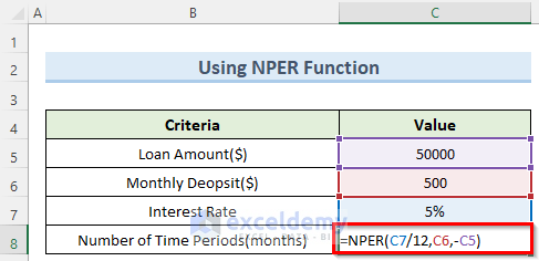
- Finally, press Enter and the formula will calculate the time periods required in months.
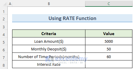
5. Utilizing RATE Function
The RATE function is used to calculate the rate charged on a loan at a constant annuity in Excel. It can also find out the rate of return needed to cover a certain amount of an investment over a given period. Let us see this function in action.
Steps:
- First, navigate to cells C5, C6, and C7 and enter the appropriate data in each one of them.
- Next, click 2 times on cell C8 and type in the below formula:
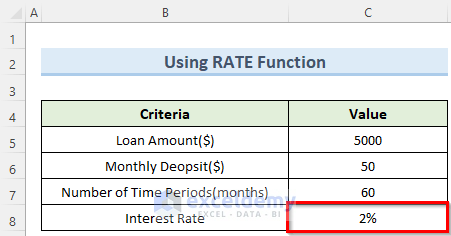
=-RATE(C7,-C6,C5)- Note here that there is a negative sign before the second parameter of this formula. This is because we are giving away money as a monthly deposit.
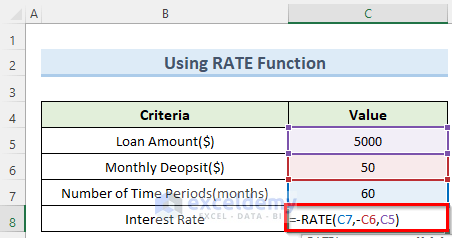
- Finally, press the Enter key, and Excel will calculate the required interest rate.
Download Practice Workbook
You can download the practice workbook from here.
Conclusion
I really hope that you found the methods that I showed in this tutorial on how to calculate annuity in Excel to be useful. I would suggest downloading the practice workbook and experimenting with different values for the required parameters. Lastly, If you have any queries, please let me know in the comments.
Excel Annuity Formula: Knowledge Hub
- How to Calculate Equivalent Annual Annuity in Excel
- How to Calculate Deferred Annuity in Excel
- How to Do Ordinary Annuity in Excel
- How to Calculate Annuity Payments in Excel
- How to Calculate Annuity Due in Excel
- How to Calculate Growing Annuity in Excel
- How to Calculate Annuity Factor in Excel
<< Go Back to Excel Formulas for Finance | Excel for Finance | Learn Excel
Get FREE Advanced Excel Exercises with Solutions!
