Whenever working with Excel, relative cell reference is frequently used. There are various uses of relative cell reference in Excel. The main objective of this article is to explain how to use relative cell reference in Excel.
What Is Relative Cell Reference?
In Excel, a relative cell reference denotes the application of a point of reference to a cell or formula where the return value is positioned in relation to the cell.
Thus, the return value changes based on whether the cell or the formula is moved inside the same sheet or to a different sheet when the cell or the formula is moved.
When the same computation must be performed across various rows or columns, relative cell reference can be useful.
How to Use Relative Cell Reference in Excel: 5 Suitable Examples
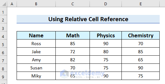
To explain this article, I have taken the following dataset. This dataset contains student’s Name and marks in different subjects like Math, Physics, and Chemistry.
1. Use of Relative Cell Reference to Copy Formula in Columns
In this first example, I will show you how to use relative cell reference in Excel for copying formulas in columns.
Let’s see the steps.
Steps:
- Firstly, select the cell where you want to calculate the Total marks. Here, I selected cell F5.
- Secondly, in cell F5 write the following formula.
=SUM(C5:E5) 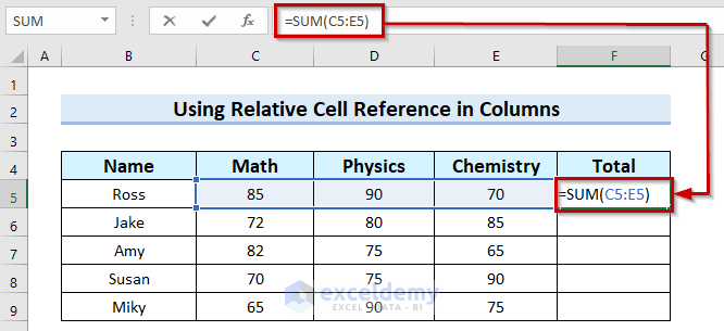
Here, the SUM function will return the summation of the values in the cell range C5:E5. In this function, I used relative cell reference to enter the cell range.
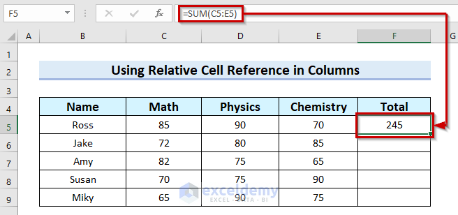
- Thirdly, press ENTER to get the result.
- Now, drag the Fill Handle to copy the formula.
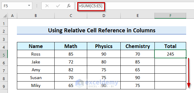
Here, I have copied the formula successfully. You can see that the cell range changed accordingly as I copied the formula. This happened because I used a relative cell reference to enter the data.
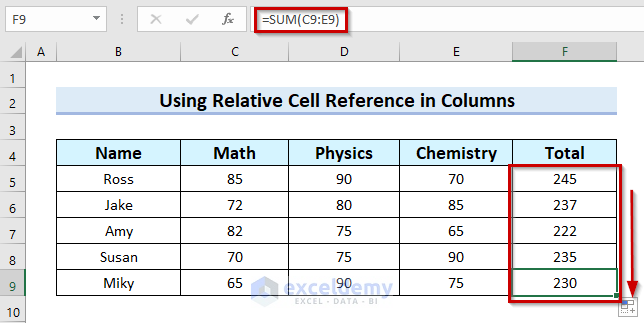
Now, I used absolute cell reference while selecting the range like the following Image.
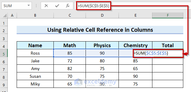
Here, the SUM function will return the summation of the values in the cell range C5:E5 and the absolute cell reference will fix this range.
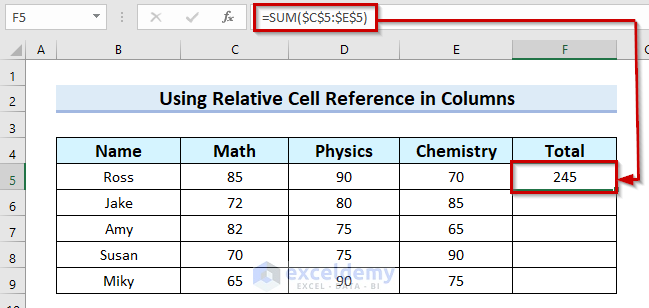
- Now, press ENTER and you will get your result.
You can see the result I got here is correct.
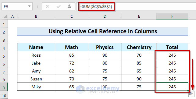
- After that, drag the Fill Handle and copy the formula.
You can see after copying the formula the result remains the same as the cell range remains the same. This is the reason, I used relative cell references before.
2. Using Relative Cell Reference to Copy Formula in Rows
In this method, I will show you how to use a relative cell reference in Excel while copying formulas in rows. I will explain 2 different examples here.
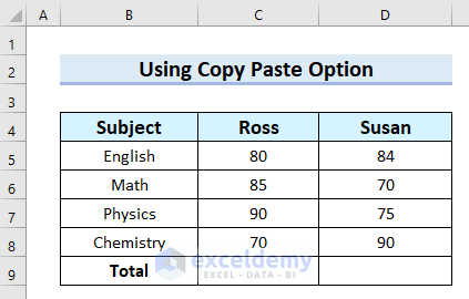
Example-01: Use of Copy Paste Option
In this example, I will use the Copy Paste option to copy formulas in rows. To Explain this example I have taken the following dataset.
Let’s see the steps.
Steps:
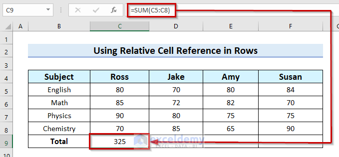
- Firstly, select the cell where you want your Total marks. Here, I selected cell C9.
- Secondly, in cell C9 write the following formula.
=SUM(C5:C8)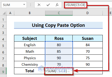
Here, the SUM function will return the summation of the values in cell range C5:C8. In this function, I used relative cell reference to enter the cell range.
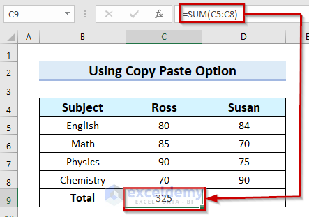
- Thirdly, press ENTER to get the result.
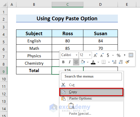
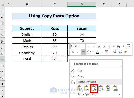
- Now, Right-click on the cell that contains the formula.
- Next, select Copy.
- After that, right-click on the cell where you want your formula to be copied.
- Then, select Formulas from Paste Options.
Now, you will see that the formula will be copied and the cell reference will change accordingly as I used relative cell reference while selecting the range.
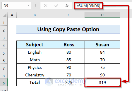
You can use this copy-paste option to copy formulas when you are copying formulas in only one or two cells. In other cases, this method is not that effective.
Example-02: Using Fill Handle
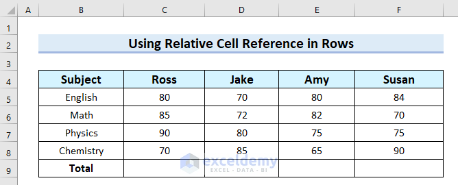
In this example, I will use the Fill Handle to copy formulas in rows. To Explain this example I have taken the following dataset.
Let’s see the steps.
Steps:
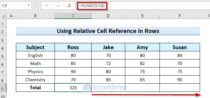
- Firstly, select the cell where you want the Total marks. Here, I selected cell C9.
- Secondly, in cell C9 write the following formula.
=SUM(C5:C8)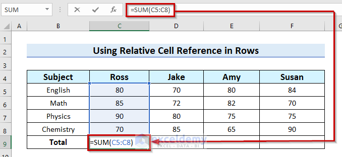
Here, the SUM function will return the summation of the values in cell range C5:C8. In this function, I used relative cell reference to enter the cell range.
- Next, press ENTER to get the result.
- Finally, drag the Fill Handle to copy the formula.
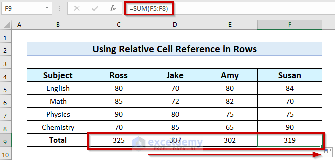
Now, you can see that I have copied the formula and the cell range changed accordingly as I used relative cell reference while selecting the cell range.
Read More: Relative Cell Reference Example in Excel
3. Use of Relative Cell Reference for Calculations
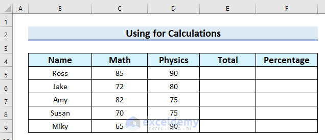
In this method, I will show you how to use a relative cell reference in Excel for calculations. Here, I have taken the following dataset to explain this example. It contains the student’s Name and marks in Math, and Physics. I will calculate the Total and Percentage using relative cell reference.
Let’s see the steps.
Steps:
- Firstly, select the cell where you want your first Total marks. Here, I selected cell E5.
- Secondly, in cell E5 write the following formula.
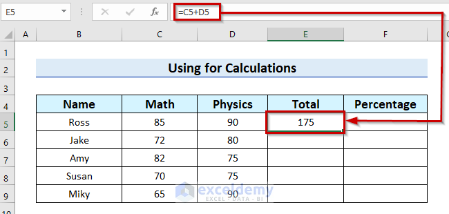
=C5+D5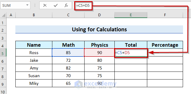
Here, I summed C5 and D5. The formula will return the summation of cells C5 and D5. I used relative cell reference while selecting the cells.
- Finally, press ENTER to get the result.
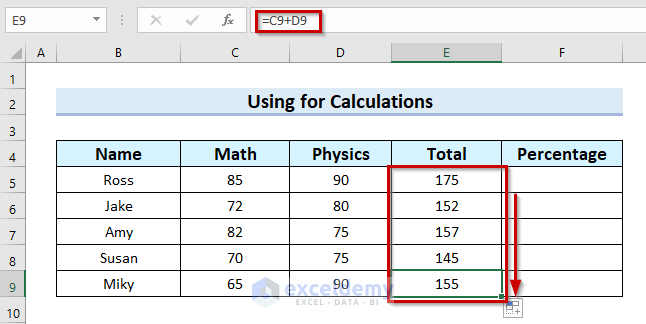
- Now, drag the Fill Handle to copy the formula to all the other cells.
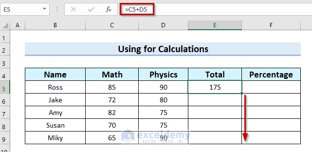
Here, you can see that I have copied the formula to all the other cells. And, the cells have changed accordingly because I used relative cell reference while selecting the cells.
Now, I will calculate the Percentage.
- Firstly, select the cell where you want to calculate the Percentage. Here, I selected cell F5.
- Secondly, in cell F5 write the following formula.
=E5/200*100%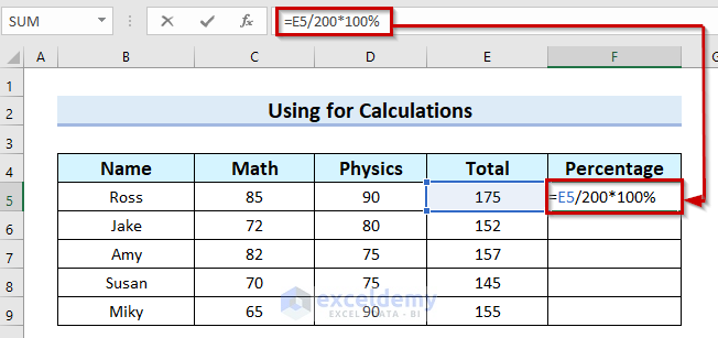
Here, I divided E5 by 200 and then multiplied the result by 100%. The formula will return the number percentage. I used relative cell reference in this case also.
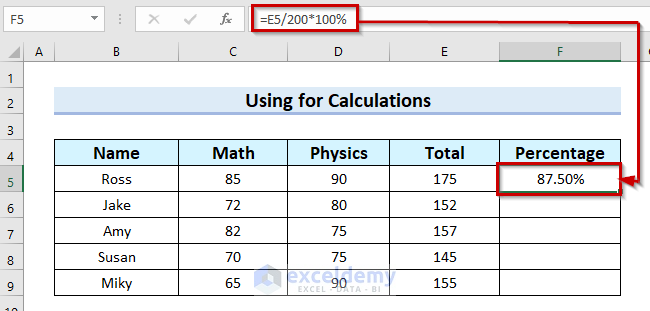
- Finally, press ENTER.
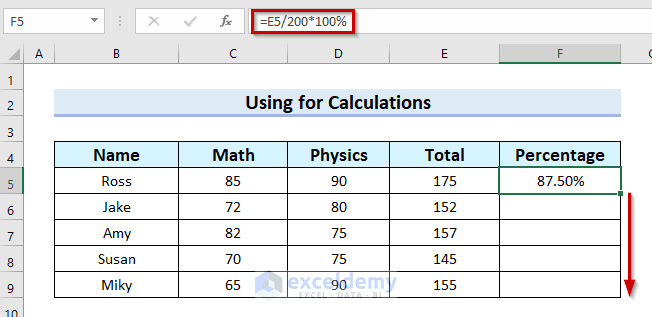
- After that, drag the Fill Handle to copy the formula.
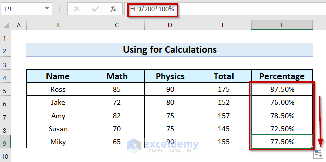
Now, you can see that I have copied the formula. Here, the cell changes accordingly.
Read More: Excel VBA: Insert Formula with Relative Reference
4. Employing Relative Cell Reference in Functions
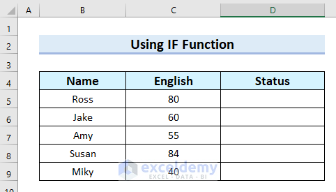
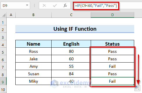
In this example, I will show you how to use a relative cell reference in Excel in functions. For this example, I have taken the following dataset. This dataset contains Name and marks in English. Here, I will show the Status as Pass or Fail.
Let’s see how it is done.
Steps:
- Firstly, select the cell where you want to show your Status. Here, I selected cell D5.
- Secondly, in cell D5 write the following formula.
=IF(C5<60,"Fail","Pass")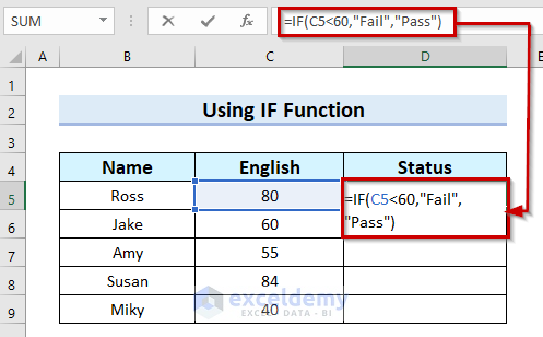
Here, in the IF function, I selected C5<60 as logical_test, “Fail” as value_if_true and “Pass” as value_if_false. The formula will return Fail if the mark is less than 60 otherwise it will return Pass. I used relative cell reference while selecting the cell.
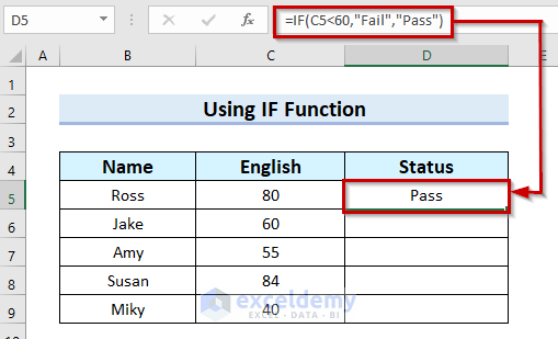
- Finally, press ENTER.
- After that, drag the Fill Handle to copy the formula
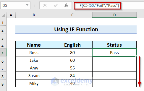
Now, you can see that I have copied the formula and the cell has changed accordingly as I use relative cell reference while selecting it.
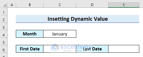
5. Using Relative Cell Reference to Insert Dynamic Value
In this method, I will explain how to use a relative cell reference to insert dynamic values. Here, I have taken the following dataset. I will use a relative cell reference to insert the First Date and Last Date.
Let’s see the steps.
Steps:
- Firstly, select the cell where you want your First Date. Here, I selected cell C6.
- Secondly, in cell C6 write the following formula.
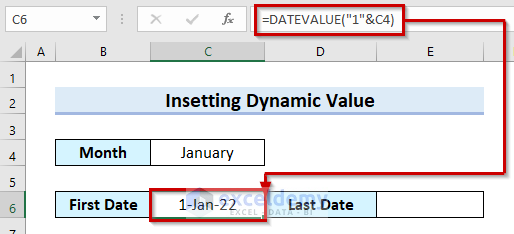
=DATEVALUE("1"&C4)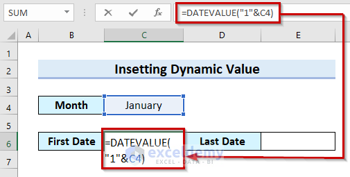
Here, in the DATEVALUE function, I used “1” and C4 as date_text. Thus, the formula will return the First Date of the month that is in cell C4. I used relative cell reference for selecting cells.
- Finally, press ENTER.
Now, I will insert the Last Date.
- Firstly, select the cell where you want your Last Date. Here, I selected cell E6.
- Secondly, in cell E6 write the following formula.
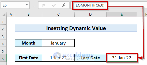
=EOMONTH(C6,0)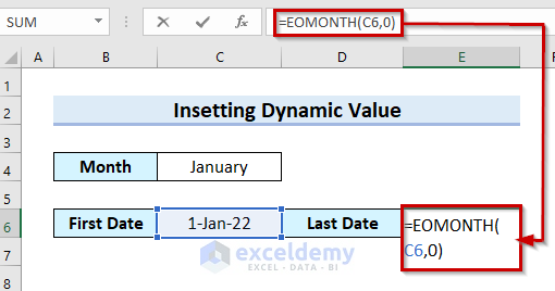
Here, in the EOMONTH function, I selected cell C6 as start_date and 0 as months. The formula will return the Last date for the month.
- Finally, press ENTER to get the result.
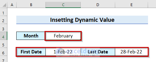
Now, If you change the Month name here the First Date and Last Date will change automatically. In the following picture, you can see that I have selected February as the month and the First Date and Last Date update automatically as I changed the month. This happens because I used relative cell reference in the formula.
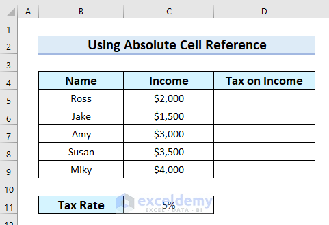
How to Use Absolute Cell Reference
In this section, I will show you how you can use an absolute cell reference. I have taken the following dataset to explain this example.
Let’s see the steps.
Steps:
- Firstly, select the cell where you want to calculate the Tax on Income. Here, I selected cell D5.
- Secondly, in cell D5 write the following formula.
=C5*C11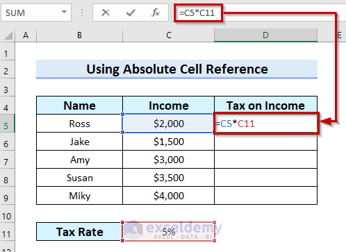
Here, I multiplied cell C5 by cell C11. The formula will return the Tax on Income by multiplying Income and Tax Rate.
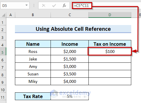
- Finally, press ENTER.
- Now, drag the Fill Handle to copy the formula.

In the following image, you can see that the result is not correct. The reason behind this is, that the cell changes accordingly as I copied the formula. This happens because I used relative cell reference while selecting cells.
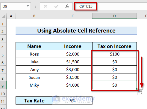
Here, you will need to use an absolute cell reference to make cell C11 fixed.
- Firstly, select the cell where you want to calculate the Tax on Income. Here, I selected cell D5.
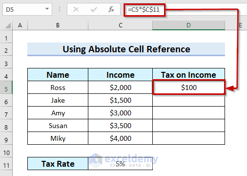
- Secondly, in cell D5 write the following formula.
=C5*$C$11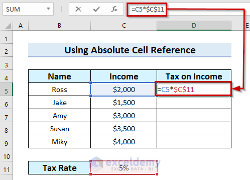
Here, I multiplied cell C5 by cell C11. The formula will return the Tax on Income by multiplying Income and Tax Rate. I used an absolute cell reference while selecting cell C11.
- Finally, press ENTER to get the result.
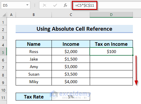
- Now, drag the Fill Handle to copy the formula.
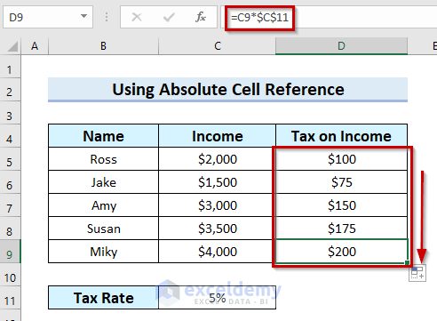
In the following image, you can see that I have copied the formula and cell C11 remains fixed because of the absolute cell reference.
Things to Remember
- It should be noted that the copy-paste method is suitable for a small set of data where you need to copy the formula to 1 or 2 cells. For big datasets using Fill Handle is more appropriate.
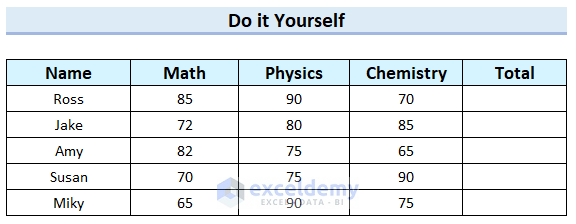
Practice Section
Here, I have provided practice for you to practice how to use relative cell reference in Excel.
Download Practice Workbook
Conclusion
In this article, I tried to explain how to use relative cell reference in Excel. I explained it with different examples. I hope this article was helpful to you. If you have any questions, feel free to let me know in the comment section below.
Related Article
<< Go Back to Relative Cell Reference | Cell Reference in Excel | Excel Formulas | Learn Excel
Get FREE Advanced Excel Exercises with Solutions!
