When working with financial data in Excel, the comma style is necessary, since adding commas between the digits makes it easier to understand the data, especially large numbers. Granted this, in this lesson, we’ll demonstrate 4 easy ways how to change comma style in Excel. In addition, we’ll also discuss how you may apply commas in Indian style and convert lakhs to millions.
How to Change Comma Style in Excel: 4 Ways
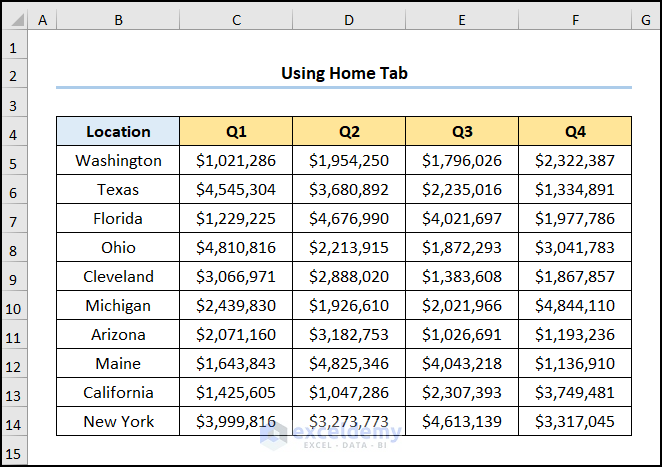
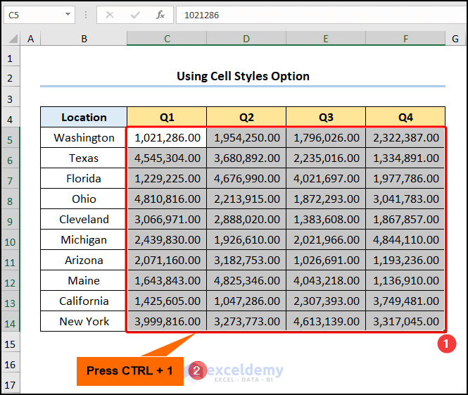
Now, let us consider the Quarterly Sales Data for 2021 dataset in the B4:F14 cells which shows the Location and the sales amount for four quarters: Q1, Q2, Q3, and Q4. As evident in the picture below, the sales values do not have commas or any currency symbols. Therefore, let’s see detailed steps for each of the methods on how to change comma style and apply currency symbols.
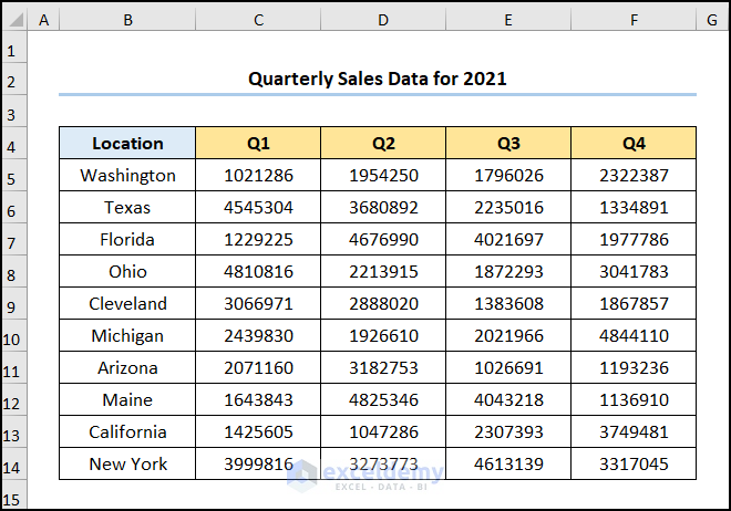
Here, we have used Microsoft Excel 365 version, you may use any other version according to your convenience.
Method-1: Using Home Tab
Let us start with the most obvious way to change comma style, simply put, using the Comma Style option in the Home tab. Here, we’ll put commas between the sales values and then format them as currency. So, let’s see it in action.
📌 Steps:
- At the very beginning, select the C5:F14 cells >> click the Comma Style button.
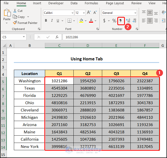
Now, this puts commas after 3 digits (1000 separator).
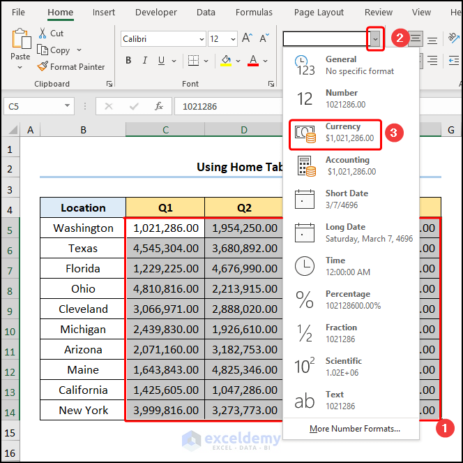
- Next, click the Number Format drop-down >> choose the Currency option.
Immediately, press the Decrease Decimal button two times to decrease the decimal place to zero.
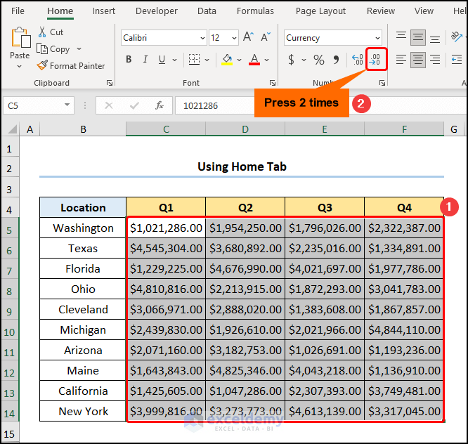
Finally, the result should look like the image given below.
Read More: How to Put Comma After 5 Digits in Excel
Method-2: Utilizing Format Cells Option
Alternatively, you can use the Format Cells option to change the comma style and apply formatting to cells. Similar to the previous method, we’ll place commas and use currency formatting for the sales amounts. Now, allow me to demonstrate the process in the steps below.
📌 Steps:
- In the first place, select the C5:F14 cells >> press CTRL + 1 on your keyboard.
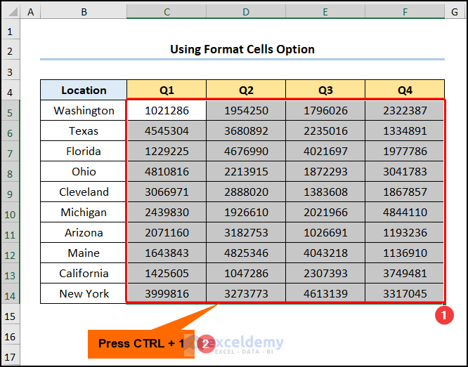
Now, this Format Cells wizard.
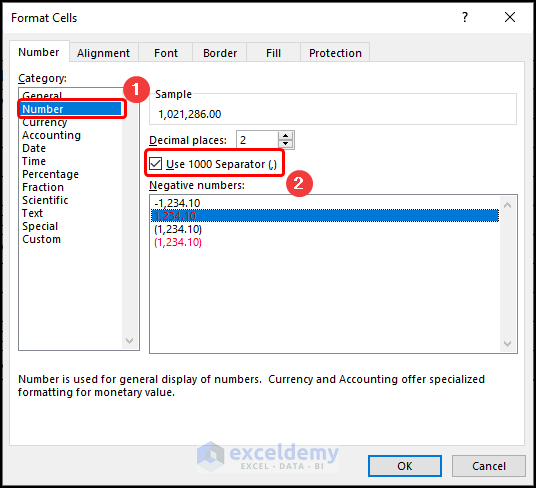
- Then, in the Category tab, select the Number option >> insert a check in the Use 1000 Separator (,) option.
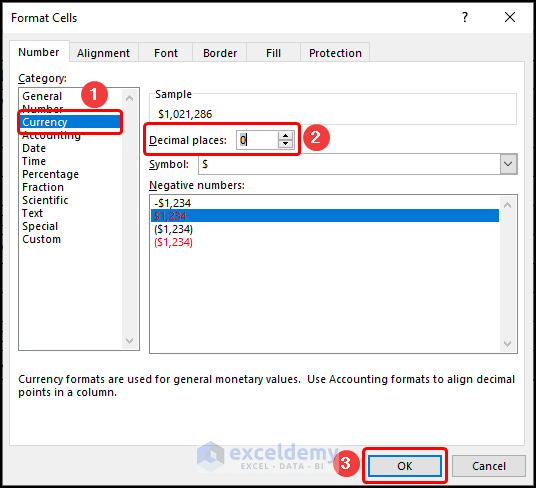
- Afterward, move to the Currency tab >> decrease the Decimal places to zero >> hit the OK button.
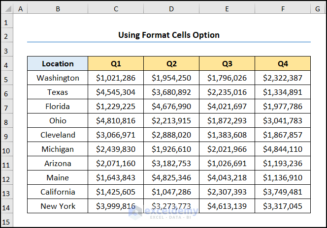
Lastly, your output should look like the screenshot given below.
Read More: How to Put Comma in Numbers in Excel
Method-3: Employing Keyboard Shortcut
If you’re wondering, are there any shortcut keys to change comma style? Then, you’re in luck because our next method answers this exact question. Hence, follow along.
📌 Steps:
- First and foremost, select the C5:F14 cells >> hit the ALT + H + K keys.
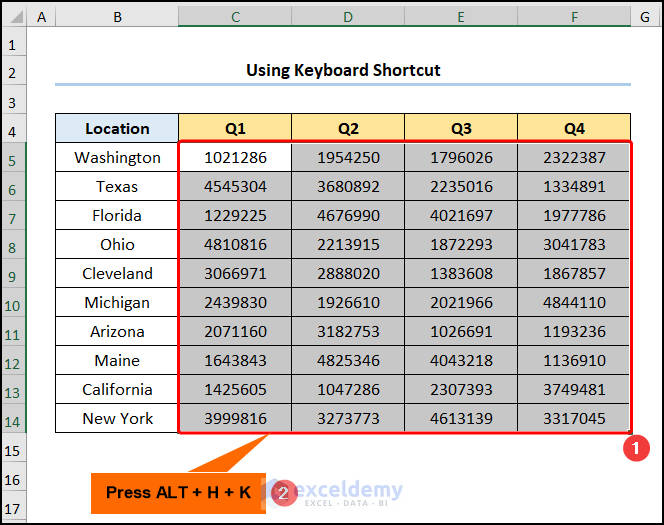
Now, this inserts commas, after 3 digits (1000 separator).
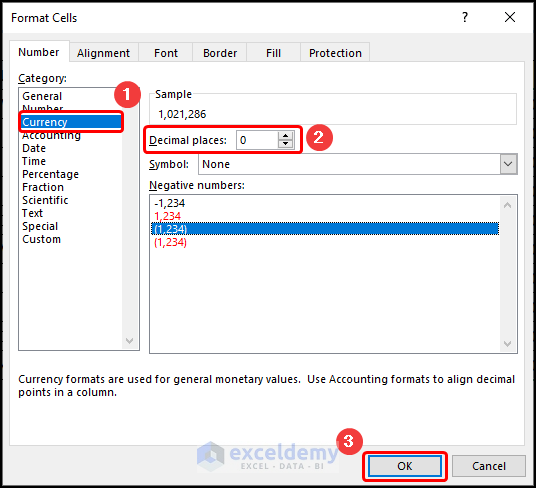
- In turn, press CTRL + 1 key to open the Number Format dialog box.

- Following this, move to the Currency tab >> decrease the Decimal places to zero >> hit the OK button.
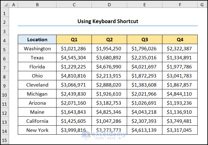
Eventually, the result should look like the picture shown below.
Method-4: Applying Cell Styles Option
Another way to change comma style involves using the Cell Style option which allows you to insert commas between numbers. So, let’s begin.
📌 Steps:
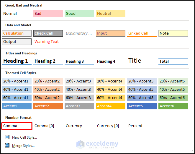
- To begin with, select the C5:F14 cells >> click the Cell Styles dropdown.

- Now, a new window appears >> select the Comma option at the bottom.
- Next, type in the keyboard shortcut CTRL + 1 to open the Format Cells dialog box.
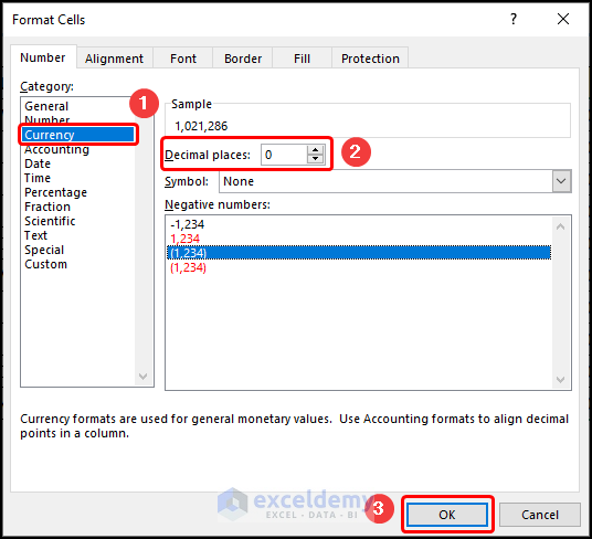
- As shown previously, choose the Currency option >> set the Decimal places to zero >> hit the OK button.
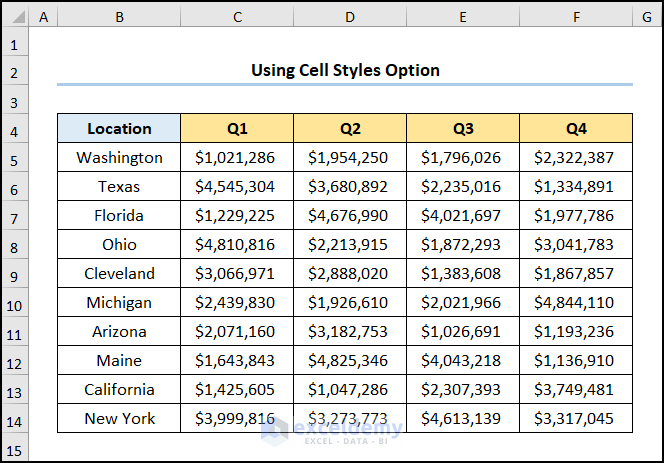
Consequently, the results should look like the screenshot given below.
Read More: [Fixed!] Style Comma Not Found in Excel
How to Change Comma Style to Indian Style in Excel
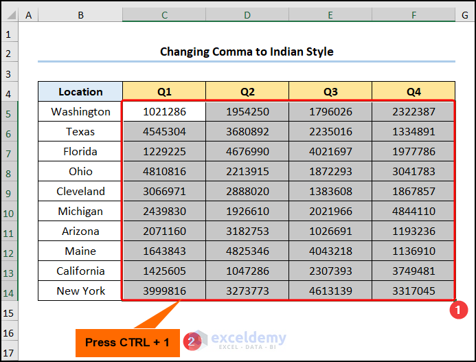
Different regions around the world use different comma types for separating numbers, for instance, a comma is added after every three digits in the US and the UK. However, in the Indian subcontinent, the Lakhs and Crores system places commas after the first three digits and then after every two digits. If you want to apply commas in the Indian style you can follow the steps described below.
📌 Steps:
- First, select the C5:F14 cells >> press CTRL + 1 on your keyboard.
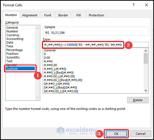
- Following this, navigate to the Custom tab >> in the Type field, enter the number format given below >> click the OK button.
[>=10000000]"RS "##\,##\,##\,##0;[>=100000]"RS " ##\,##\,##0;"RS "##,##0
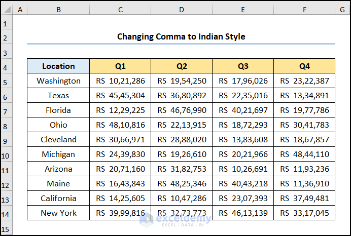
Subsequently, this should return the results as shown in the image below.
Read More: How to Change Comma in Excel to Indian Style
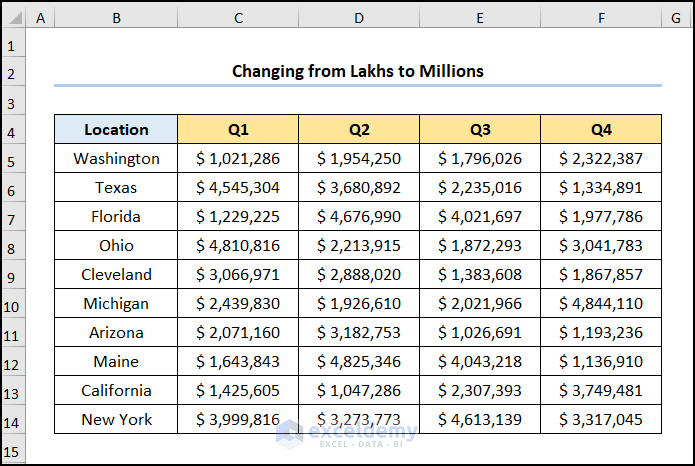
How to Change Comma Style from Lakhs to Million in Excel
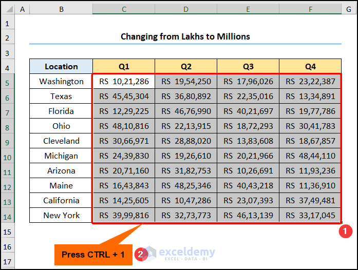
In case you want to change from Lakhs to Millions you may follow the steps shown below.
📌 Steps:
- In the first place, select the C5:F14 cells >> press CTRL + 1 on your keyboard.
- Second, move to the Custom tab >> in the Type field, enter the number format given below >> click the OK button.
$ #,##0
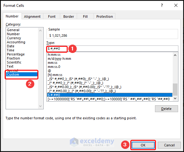
Eventually, the output should look like the picture shown below.
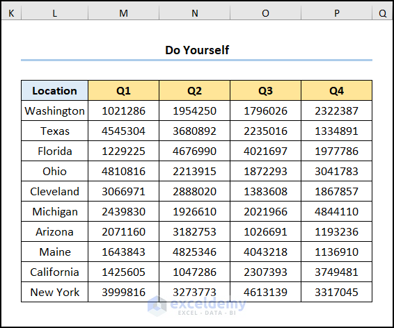
Practice Section
We have provided a Practice section on the right side of each sheet so you can practice yourself. Please make sure to do it by yourself.
Download Practice Workbook
You can download the practice workbook from the link below.
Conclusion
Last but not the least, I hope this tutorial has provided you with useful knowledge on how to change comma style in Excel. We recommend you learn and apply all these instructions to your dataset. Download the practice workbook and try these yourself. Also, feel free to give feedback in the comment section. Your valuable feedback keeps us motivated to create tutorials like this.
Related Articles
<< Go Back to How to Add Comma in Excel | Concatenate Excel | Learn Excel
Get FREE Advanced Excel Exercises with Solutions!
