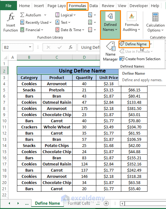
How to Highlight Selected Cells in Excel (5 Easy Ways)

Method 1 – Using Define Name to Highlight Selected Cells in Excel

Step 1: Go to Formulas Tab > Select Define Name (in Define Names section).

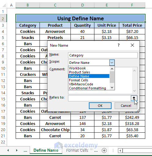
Step 2: A New Name window will open.

In the New Name window, enter a desired name (e.g., Category) in the Name
Select Define Name as Scope.
Click on the Icon next to the Refers to box to select cells or a range of cells you want to assign the Name Category

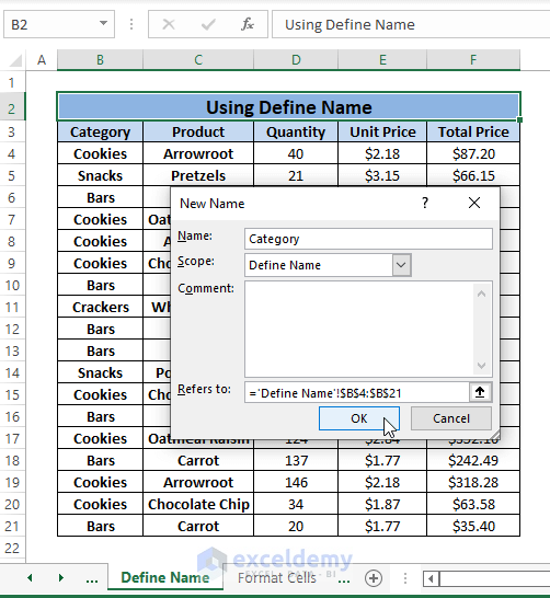
Step 3: Select the cells or range of cells (e.g., B4:B21) to define as Category.

Step 4: ENTER to return to the New Name window, then Click OK.

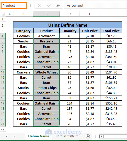
The Name Box (Left box to the Formula Bar box) will now show the assigned name.

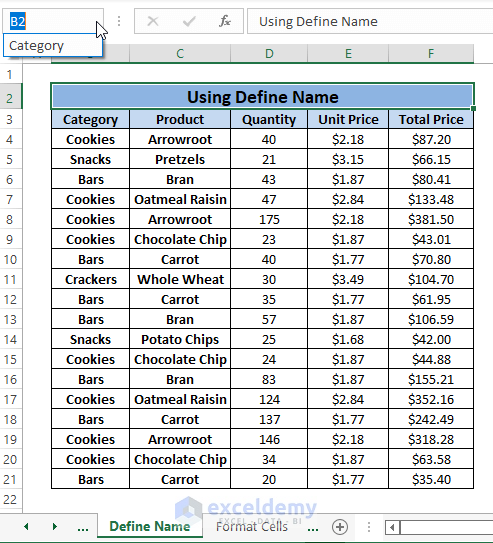
Name Box

Step 1: Select cells or a range i.e., C4:C21) of cells, then go to the Name Box and type any Name (i.e., Product) you want. Hit Enter.

Assign names as needed. Selecting a name from the Name box highlights the corresponding cells.

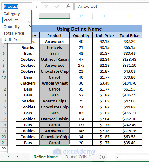
You can even assign multiple names based on your data types.

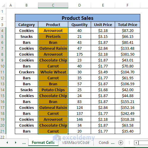
Method 2 – Applying Excel Format Cells Feature to Highlight Selected Cells

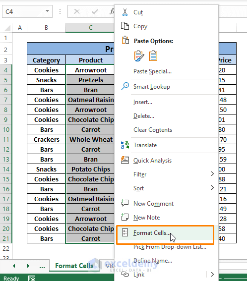
Step 1: Select cells or a range of cells and Right-Click on any of the selected cells. From the Context Menu options, select Format Cells.

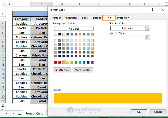
Step 2: In the Format Cells window, Select Fill as the highlighting method and Choose any color (e.g., Yellow). Click OK.

Alternatively, press Ctrl+1 to open the Format Cells window.

The selected cells or range of cells will be highlighted.

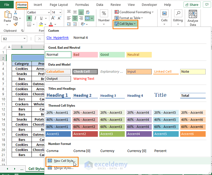
Method 3 – Using Cell Styles to Highlight Selected Cells in Excel

Step 1: Go to Home Tab > Select Cell Styles (in Styles section) > Select New Cell Style.

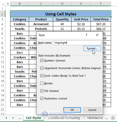
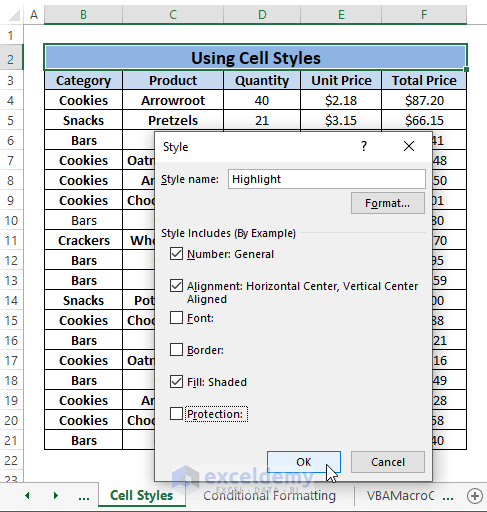
Step 2: In the Style command box, type a Style name (e.g., Highlight). Click on Format.

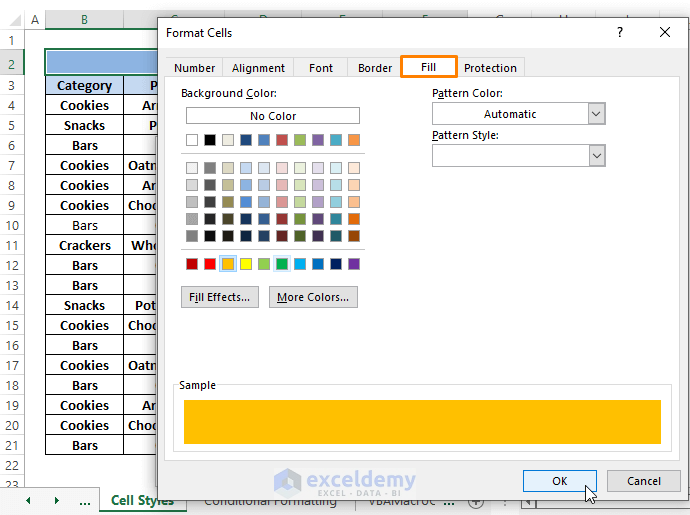
Step 3: Click on Fill, and choose any color (e.g., Yellow) to Highlight the cells. Click OK.

Step 4: Click OK on the Style dialog box.

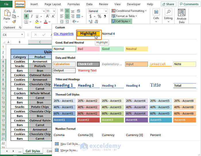
Step 5: Select a cell or a range of cells. Go to Home Tab > Select Cell Styles (in Styles section).

You’ll see a custom Highlight cell style containing all the highlight options you put into Step 3.

Click on the Highlight cell style option.

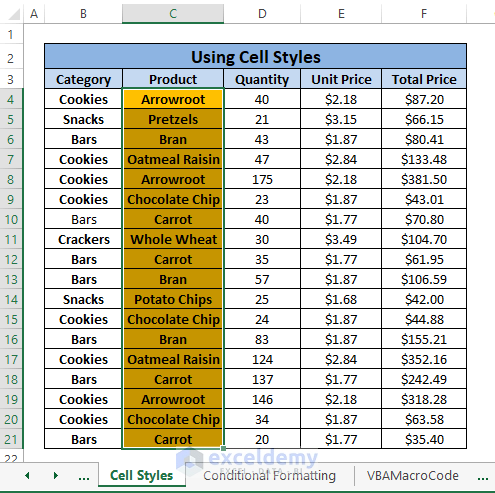
The selected cells get highlighted by the Fill color (i.e., Yellow) you chose.

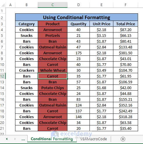
Method 4 – Using Excel Conditional Formatting to Highlight Selected Cells (Row and Column)

In this case, we can use formulas to highlight the active cell’s row and column together or individually.

Case 1: Both Row and Column in Same Color

To highlight both active cell’s rows and columns we use the OR function.

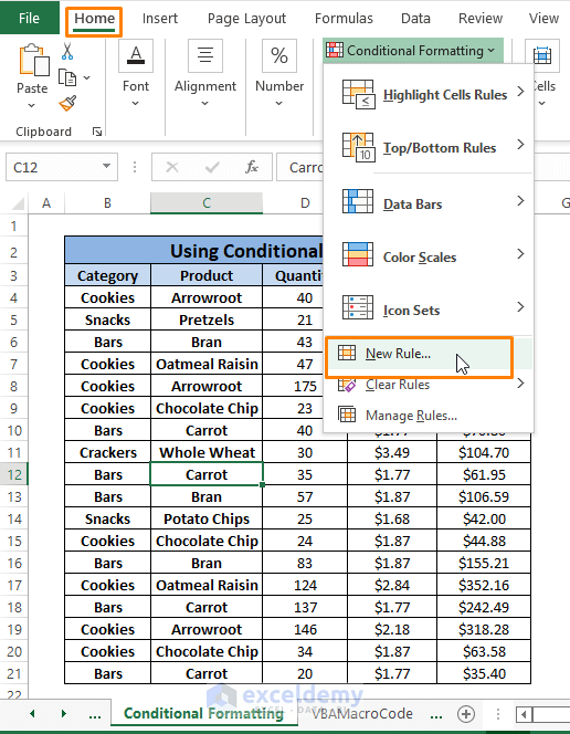
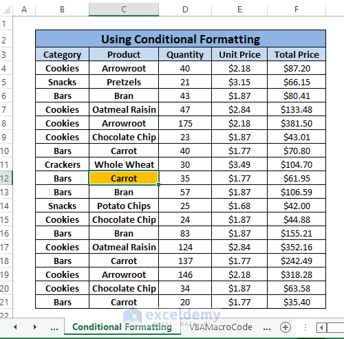
Step 1: Click on any cell (e.g., C12) for which you want to highlight both the row and column.

Go to Home Tab > Select Conditional Formatting (in Style section)> Choose New Rule.

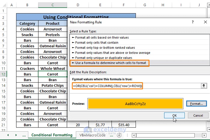
Step 2: In the New Formatting Rule window, Choose Use a formula to determine which cell to format from Select a Rule Type option.

Paste the following formula in the Edit the Rule Description box.

=OR(CELL("col")=COLUMN(),CELL("row")=ROW())

Here in the formula,

CELL(“col”)=COLUMN(); compares the selected cell’s column that is CELL(“col”) to the cell’s column to be highlighted that is COLUMN().

CELL(“row”)=ROW();compares the selected cell’s row that is CELL(“col”) to the cell’s row to be highlighted that is ROW().

We patch them with the OR function to highlight the cell’s row and column if either of the arguments is TRUE.

Follow Step 3 of Method 3 to choose the Fill color (i.e., Yellow).

Click OK.

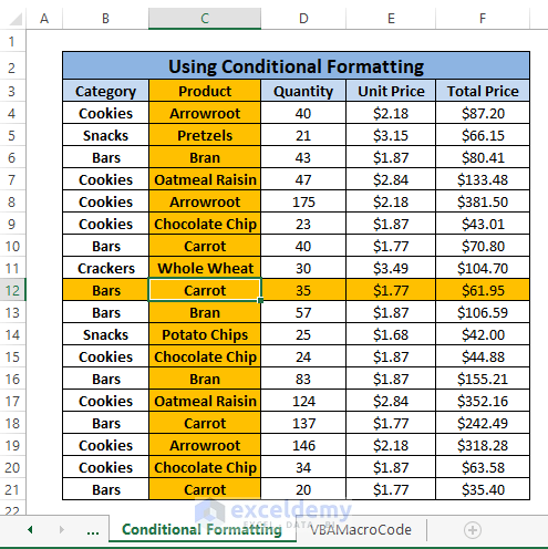
You’ll see an outcome similar to the image below.

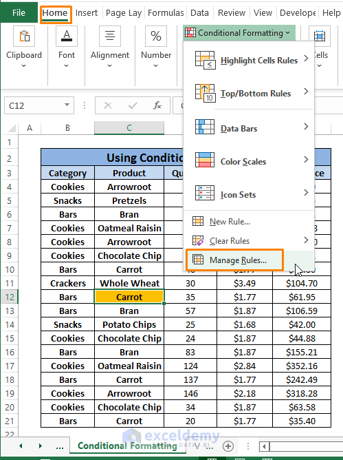
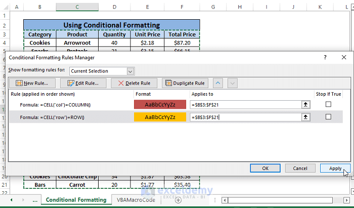
Step 3: Go to Conditional Formatting > Choose Manage Rules.

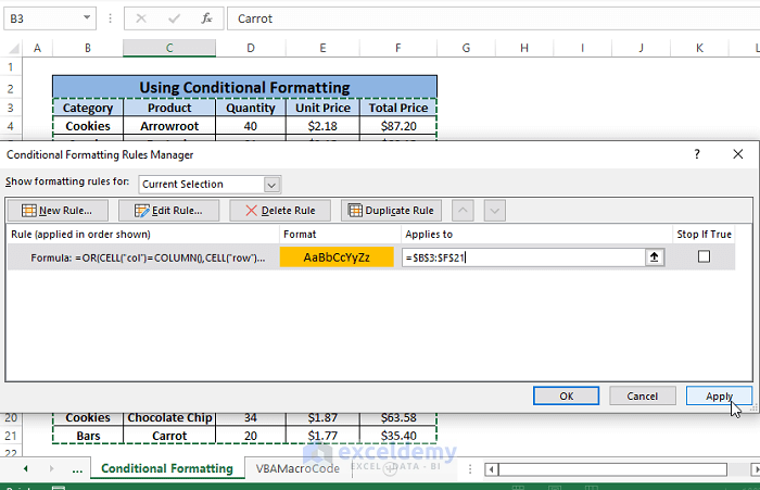
Step 4: Select the whole range (e.g., B3:H21) in the Applies to command box. Click on Apply.

The active cell’s row and column will be highlighted.

Case 2: Row and Column in Different Color

Step 1: Repeat Steps 1 to 4 of Case 1.

Replace the formula with two New Rules.

=CELL("row")=ROW()

=CELL("col")=COLUMN()

These two formulas declare the same argument as they did in Case 1.

Select two different Fill colors following Step 3 of Method 3.

Select the whole dataset to Applies to the dialog box.

Click on Apply.

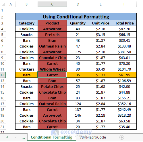
The resultant will be similar to the image below.

Case 3: Only Row or Column

Step 1: Repeat Step 1 of Case 2.

Choose any of the Fill Color as No Color. In this case, we select the row formula to highlight the row with no color.

Click on Apply.

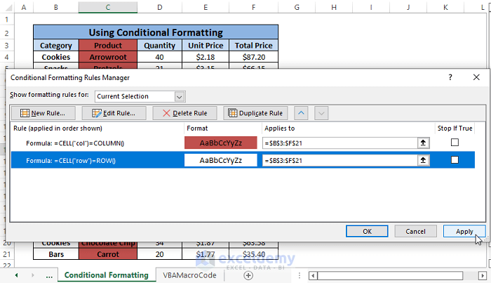
The outcome will be similar to the following image.

You can choose No Color as Fill Color for Column and the result will be the opposite.

Method 5 – Using VBA Macro Code to Highlight Selected Cells

Step 1: Press ALT+F11 to open the Visual Basic window.

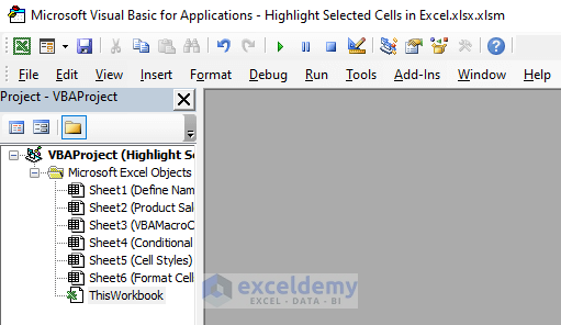
Step 2: Double-click on Sheet3 (VBAMacroCode) to bring up the Visual Basic Worksheet. Paste and save the following code in the Worksheet.

Private Sub Worksheet_SelectionChange(ByVal Target As Range)
Selection.Worksheet.Cells.FormatConditions.Delete
Selection.FormatConditions.Add xlExpression, , "TRUE"
Selection.FormatConditions(1).Interior.Color = vbYellow
End Sub

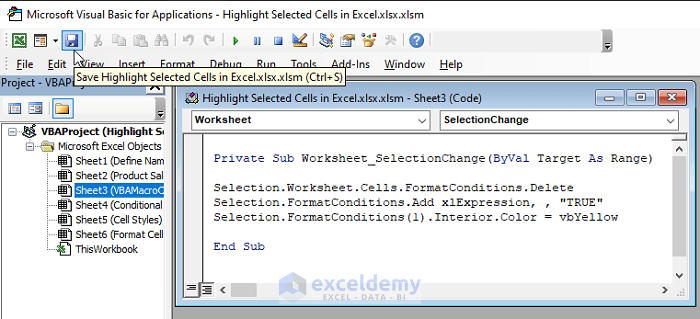
The code deletes any previous cell formats and formats any selection, particularly in Sheet3. In the code, we chose Yellow as the highlighting color. You can choose any color.

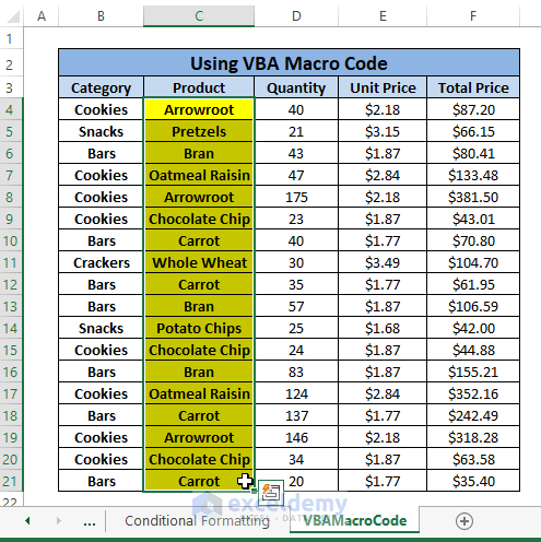
Step 3: Go back to the Excel Worksheet, select any cell or range of cells; you’ll see it simultaneously get highlighted with Yellow color.