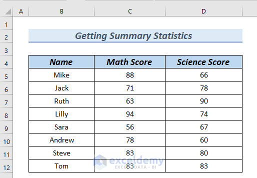
The following dataset has 3 columns (Name, Math Score, and Science Score).
Method 1 – Using the Status Bar to Get Summary Statistics in Excel
Steps:
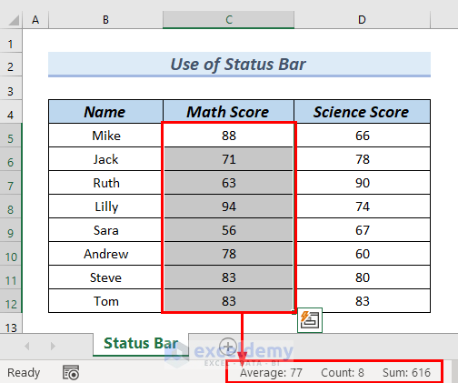
- Select C5:C12 in the Math Score column.
- In the Status Bar, you can see the Average, Count, and Sum of the selected cells.
Maximum and Minimum are missing.
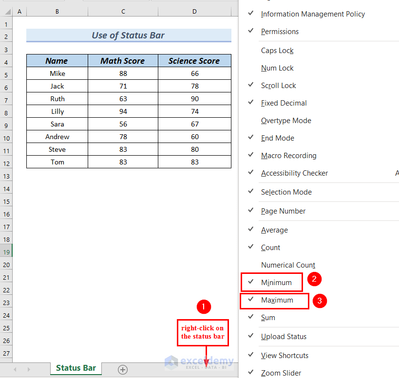
- To add Maximum and Minimum to the Status Bar, right-click it.
- Check Minimum and Maximum from the Customize Status Bar.
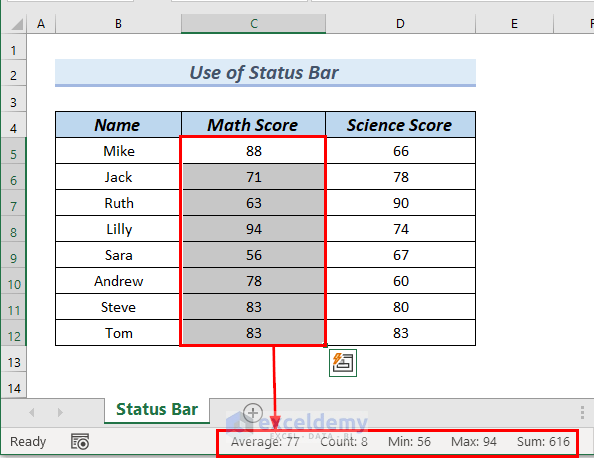
- Select C5:C12 in the Math Score column.
In the Status Bar, you can see the Average, Count, Min, Max, and Sum of the selected cells.
Method 2 – Applying the SUM, AVERAGE, MAX, MIN, and COUNT Functions
Steps:
To calculate the Sum of the Math Score:
- Enter the following formula in C16.
=SUM(C5:C12)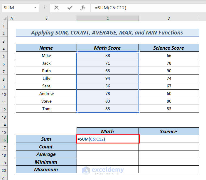
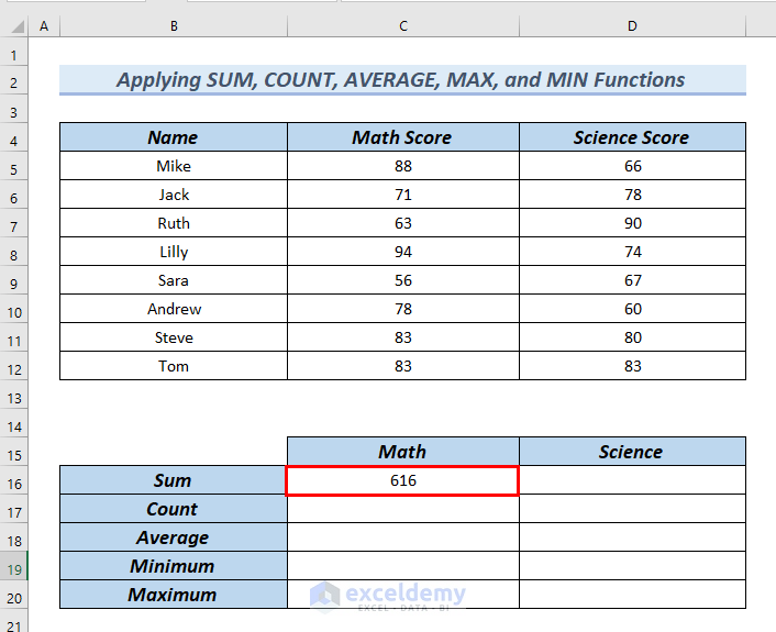
- Press ENTER.
The Sum of the Math Score is displayed in C16.
- Enter the following formula in C17 to calculate the Count of the Math Score.
=COUNT(C5:C12)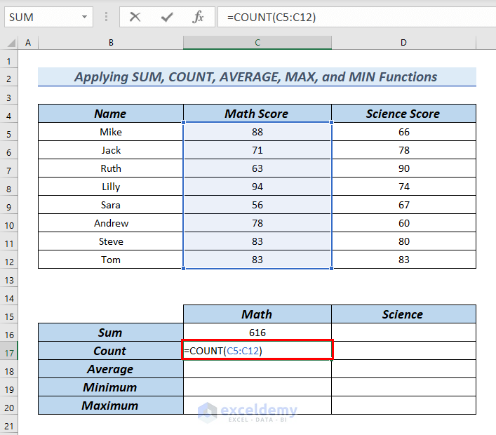
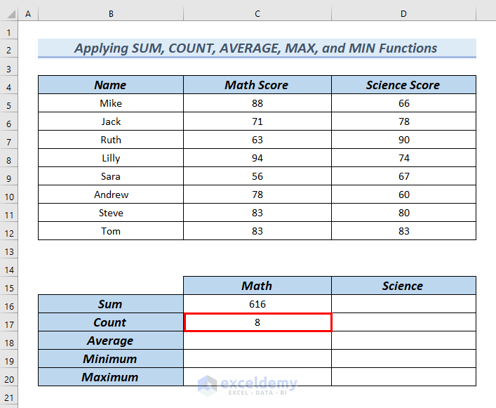
- Press ENTER.
You will see the Count of the Math Score in C17.
- Enter the following formula in C18 to calculate the Average of the Math Score.
=AVERAGE(C5:C12)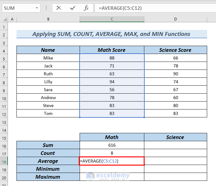
- Press ENTER.
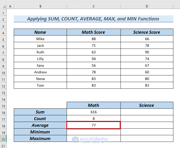
You can see the Average of the Math Score in C18.
- Enter the following formula in C19 to calculate the Minimum of the Math Score.
=MIN(C5:C12)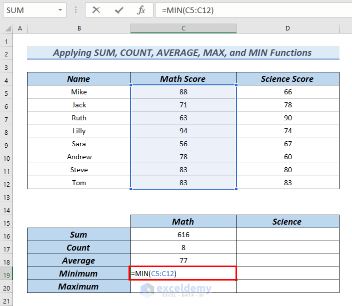
- Press ENTER.
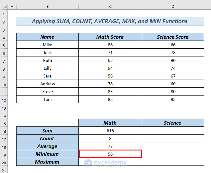
You will see the Minimum of Math Score in C19.
- Enter the following formula in C20 to calculate the Maximum of the Math Score.
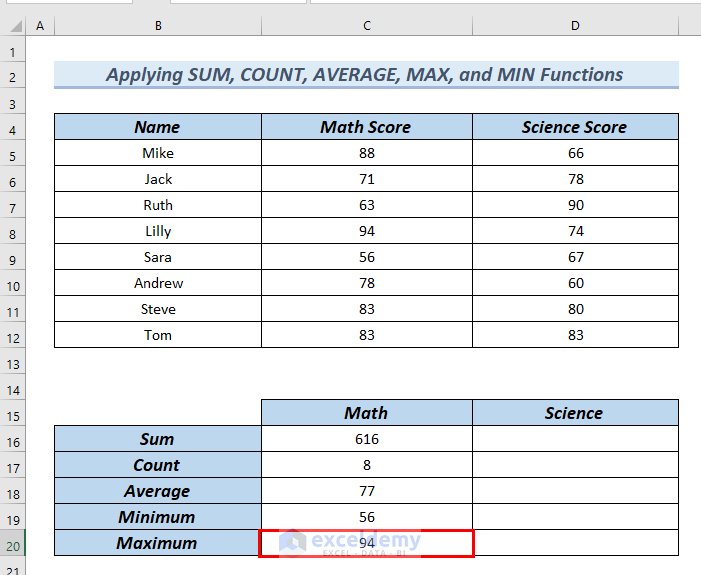
=MAX(C5:C12)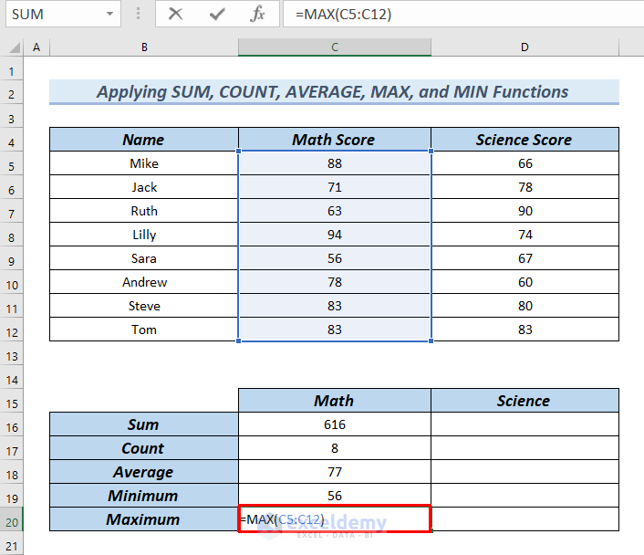
- Press ENTER.
You will see the Minimum of Math Score in C19.
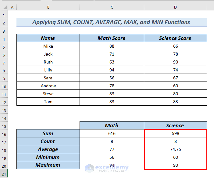
- Follow the same procedure to calculate the summary statistics of the Science column.
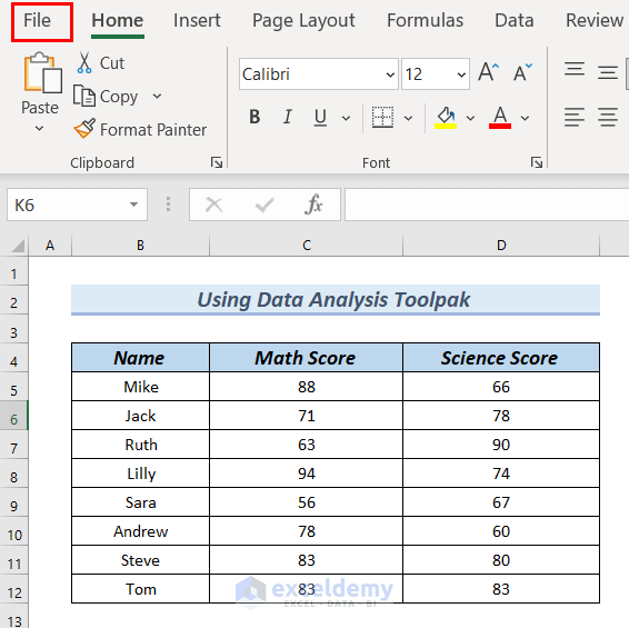
Method 3 – Using the Data Analysis ToolPak to Get Summary Statistics for One Quantity
Step1: Enabling the Analysis ToolPak
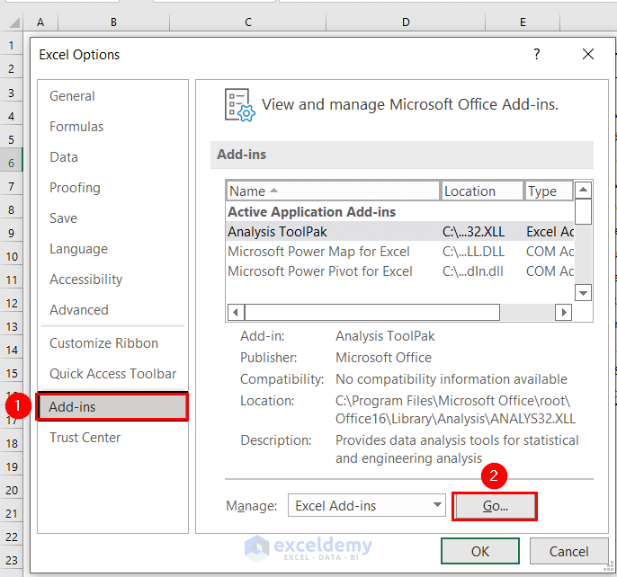
- Go to the File tab.
- Select Options.

The Excel Options dialog box will open.
- In Add-ins >> click Go.
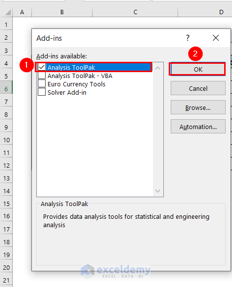
In the Add-ins dialog box:
- Check Analysis Toolpak >> click OK.
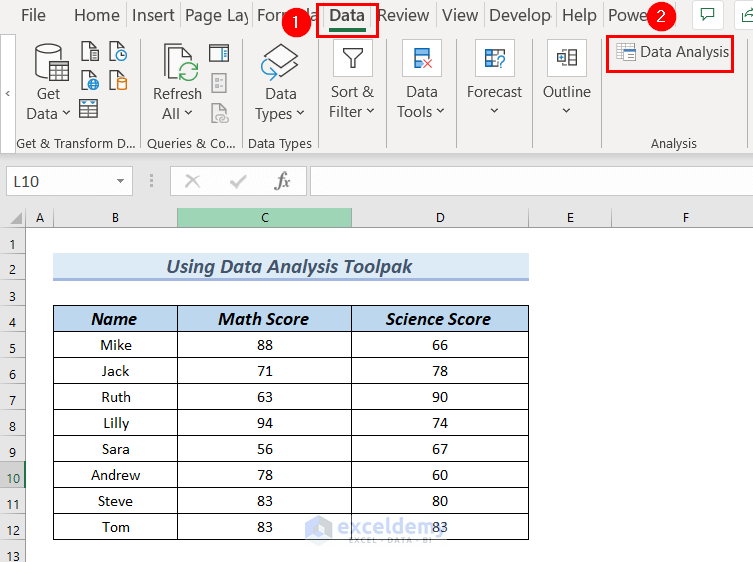
Step 2: Getting Summary Statistics Using the Data Analysis Toolpak
- In the Data tab >> select Data Analysis.
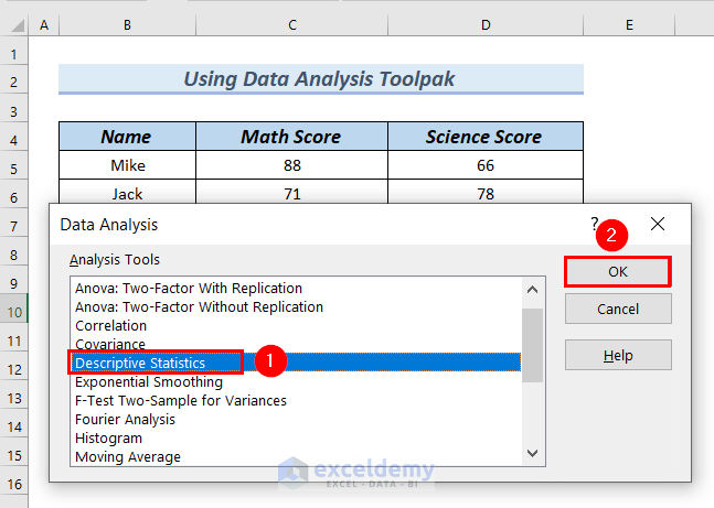
In the Data Analysis dialog box:
- In Analysis Tools >> select Descriptive Statistics.
- Click OK.
At this point, a Descriptive Statistics dialog box will appear.
- Select C4:C12 as Input Range.
- Check Labels in first row.
- In Output options, select Output Range as F2.
- Check Summary statistics.
- Click OK.
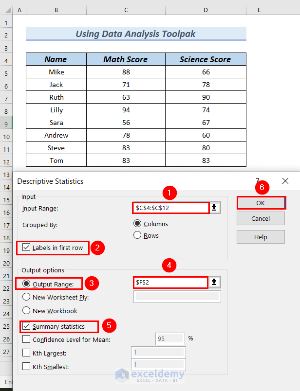
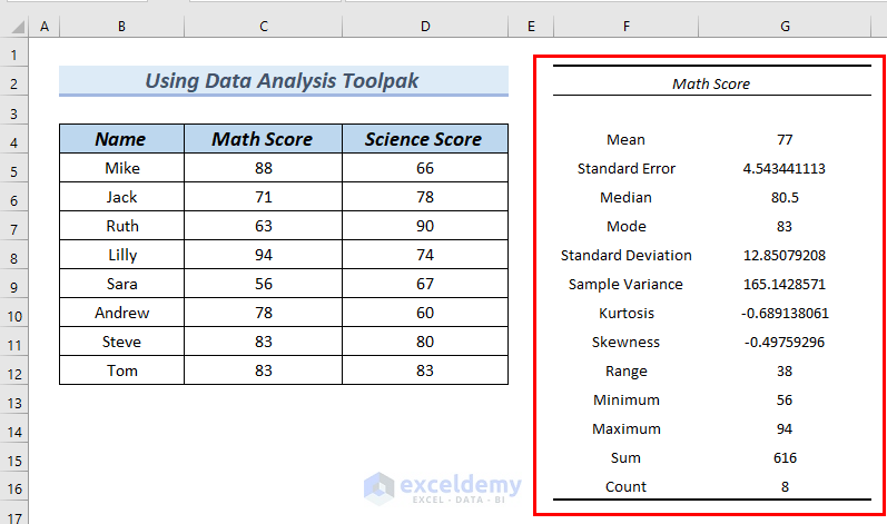
You can see the summary statistics.
Read More: Descriptive Statistics – Input Range Contains Non-Numeric Data
Method 4 – Using the Quick Analysis Feature
Step1: Applying the Quick Analysis Feature
- Go to the File tab.
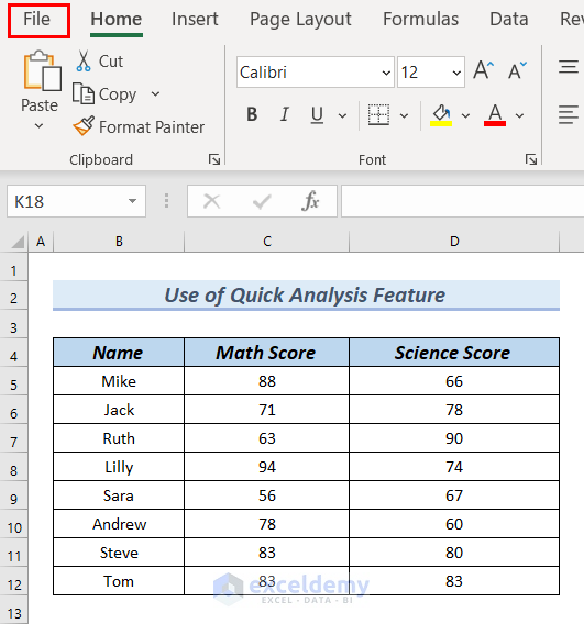
- Select Options.

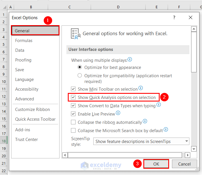
- Choose General.
- In User Interface options >> check Show Quick Analysis options on selection.
The Quick Analysis feature will be enabled.
Step 2: Obtaining a Summary Using the Quick Analysis Feature
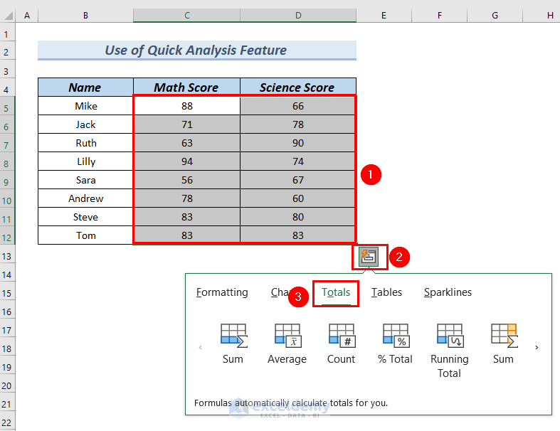
- Select C5:D12.
- Click the Quick Analysis feature on the left bottom side of the selected data (a red color box).
Select C5:D12 and press CTRL+Q to see the options.
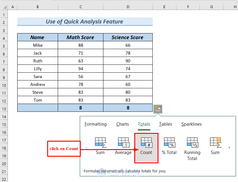
- Select Totals.
You can see the Sum, Average, and Count among other options.
- Hover your mouse on Sum to see the Sum of Math and Science Scores in C13 and D13.
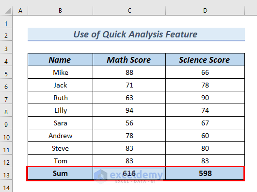
- Click Sum.
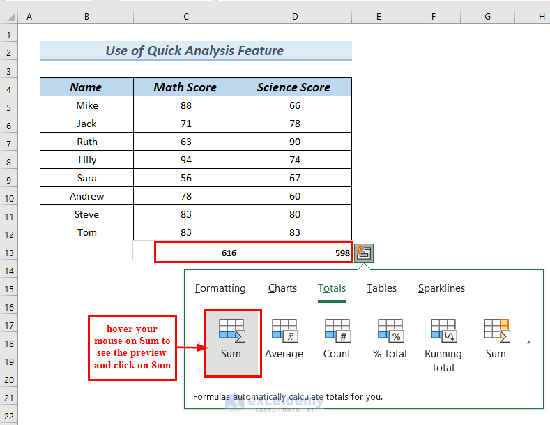
This is the output.
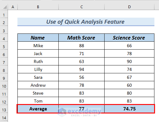
- Hover your mouse on the Average to see the Average of the Math and Science Scores in C13 and D13.
- Click Average.
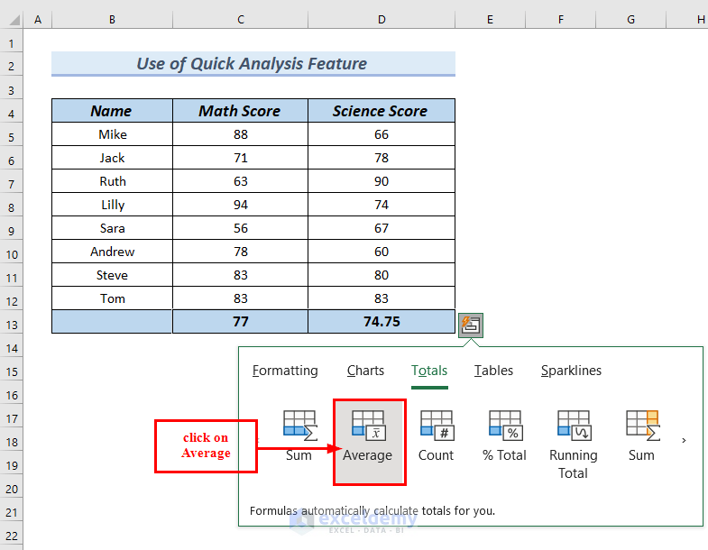
This is the output.
- Hover our mouse on the Count to see the Count of the Math and Science Scores in C13 and D13.
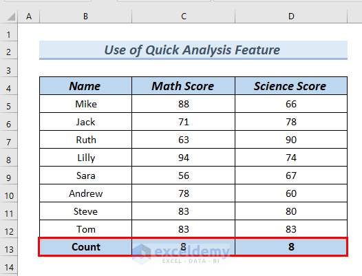
- Click Count.
This is the output.
Method 5 – Using the Table Feature to Get Summary Statistics in Excel
Step 1: Inserting the Table
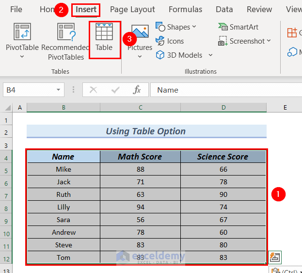
- Select the entire dataset (B4:D12) or click on B4 and press CTRL+SHIFT+Right arrow+Down arrow.
- In the Insert tab >> select Table.
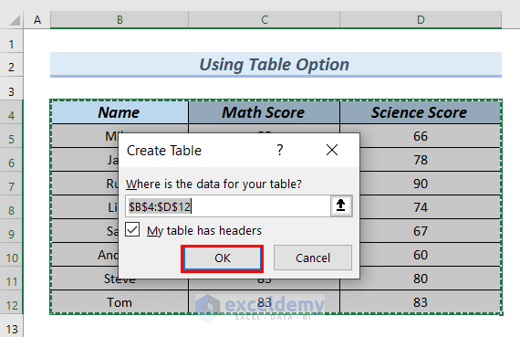
In the Create Table dialog box:
- Make sure My table has headers is checked.
- Click OK.
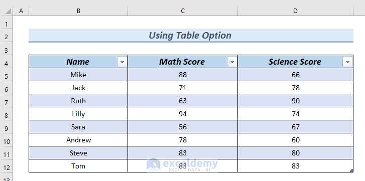
The Table is displayed.
Step 2: Getting Summary Statistics Using a Table
- Click a cell in the Table. Here, D9.
- In Table Design tab, choose Table Style Options >> select Total Row.
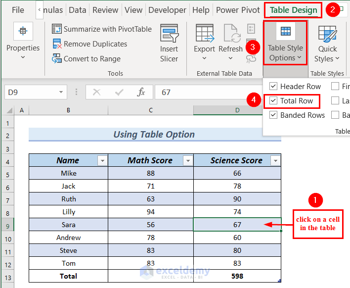
You can see the Total in D13 and two drop-down arrows in C13 and D13.
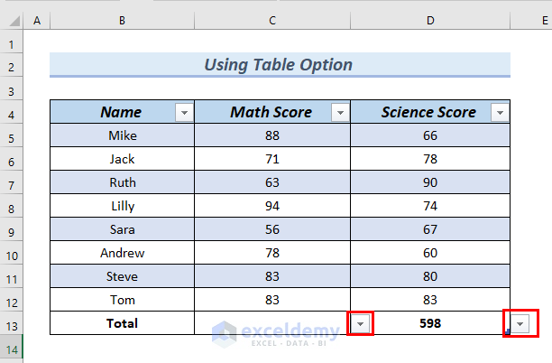
- Click the drop-down arrow in C13 to see the statistics in the drop list.
- Select Sum.
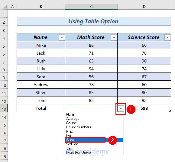
You can see the Sum of the Math Score in C13.
- Click the drop-down arrow in D13.
- Select Average.
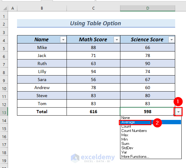
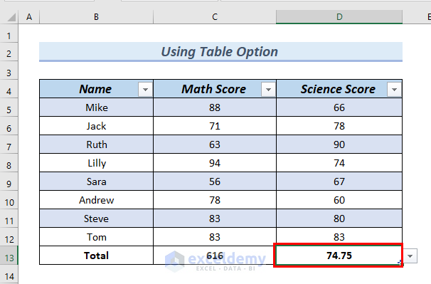
You can see the Average of the Science Score in D13.
Follow the same steps to find out other statistics.
Method 6. Inserting a Pivot Table to Get Summary Statistics in Excel
Step 1: Adding a Pivot Table
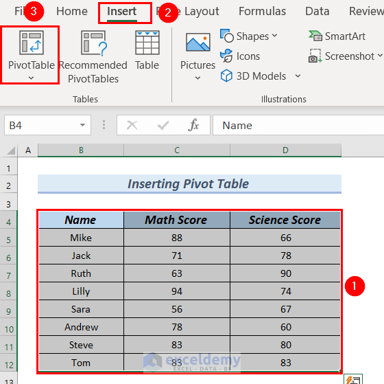
- Select the entire dataset: B4:D12.
- In the Insert tab >> select PivotTable.
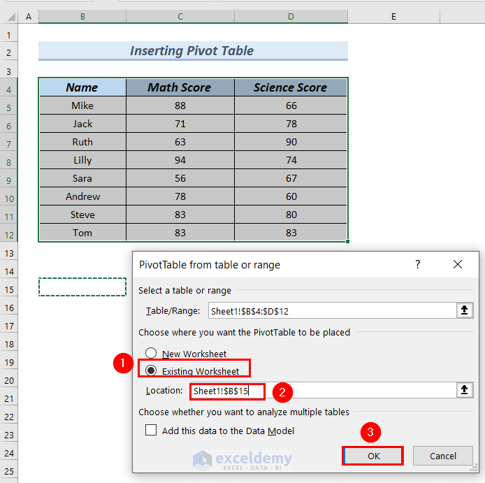
The Pivot Table from table or range dialog box will open.
- Select the Existing Worksheet.
- Select B15 as the Location.
- Click OK.
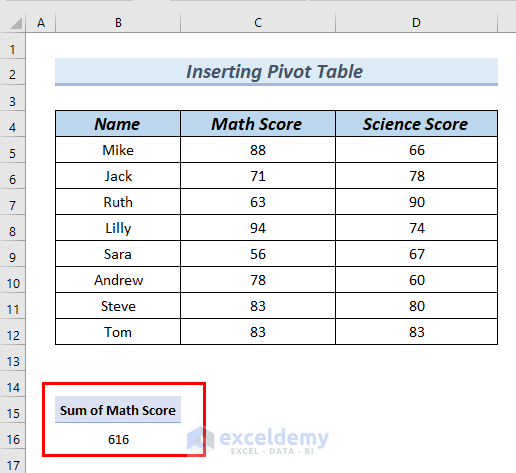
The Pivot Table will be created in the Existing Worksheet.
Step 2: Obtaining Summary Statistics Using a Pivot Table
- In PivotTable Fields >> check Math Score.
- Drag the Math Score into the Values group.
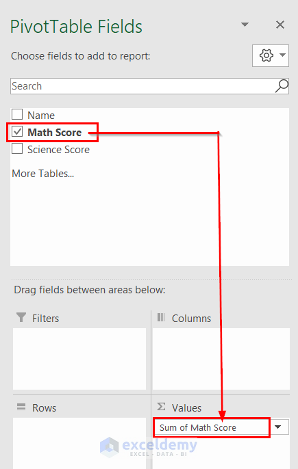
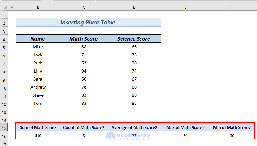
You can see the Sum of Math Score in B16.
To see the Count of the Math Score.
- In PivotTable Fields >> check Math Score.
- Drag the Math Score into the Values group.
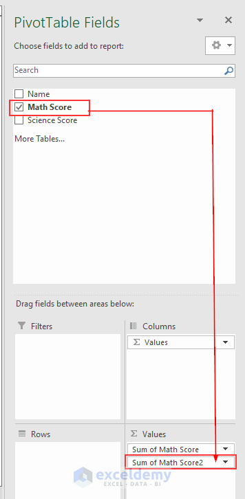
The Sum of Math Score2 is displayed in C16.
- Right-click C15 >> select Summarize Values By
- Select Count.
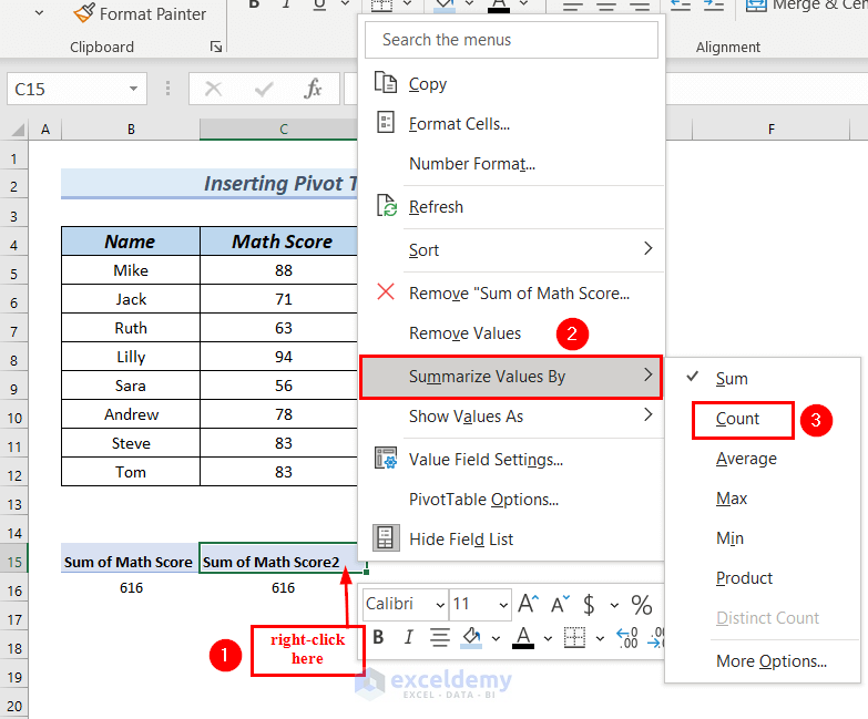
You will see the Average, Maximum, and Minimum of the Math score (the Average in D16, Max in E16, and Min in F16).
Method 7 – Using the Power Query to Get Summary Statistics in Excel
Step 1: Using the Power Query
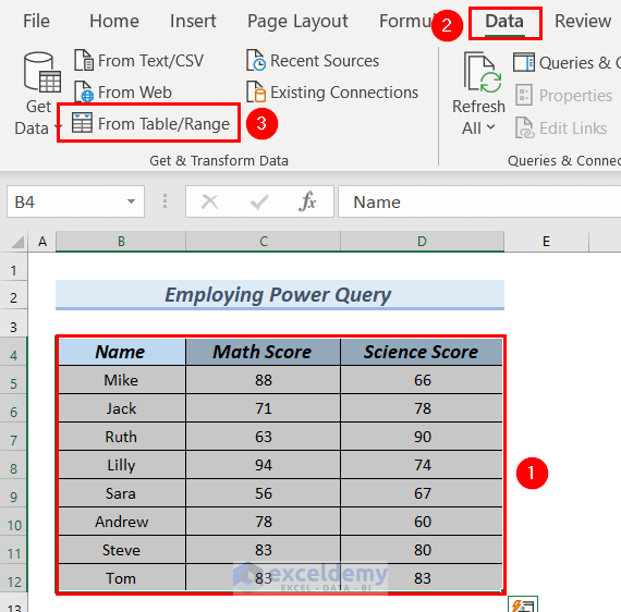
- Select the entire dataset >> go to the Data tab.
- In Get & Transform Data >> Select From Table/Range.
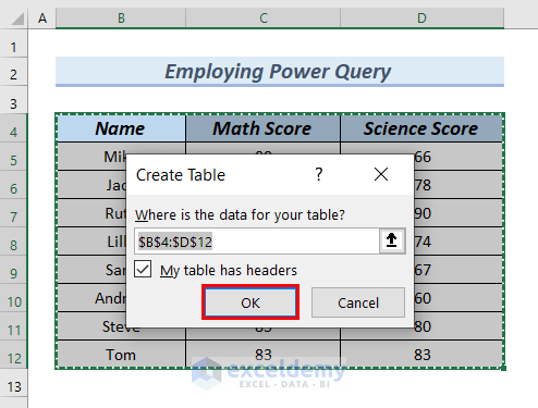
The Create Table dialog box will be displayed.
- Click OK.
The Power Query is displayed.
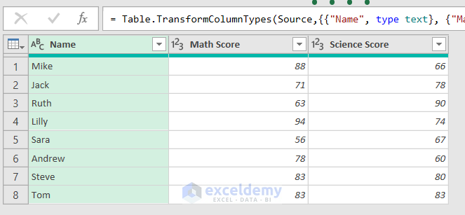
Step 2: Getting Summary Statistics Using the Power Query
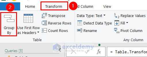
- Go to the Transform tab.
- In Table >> select Group By.
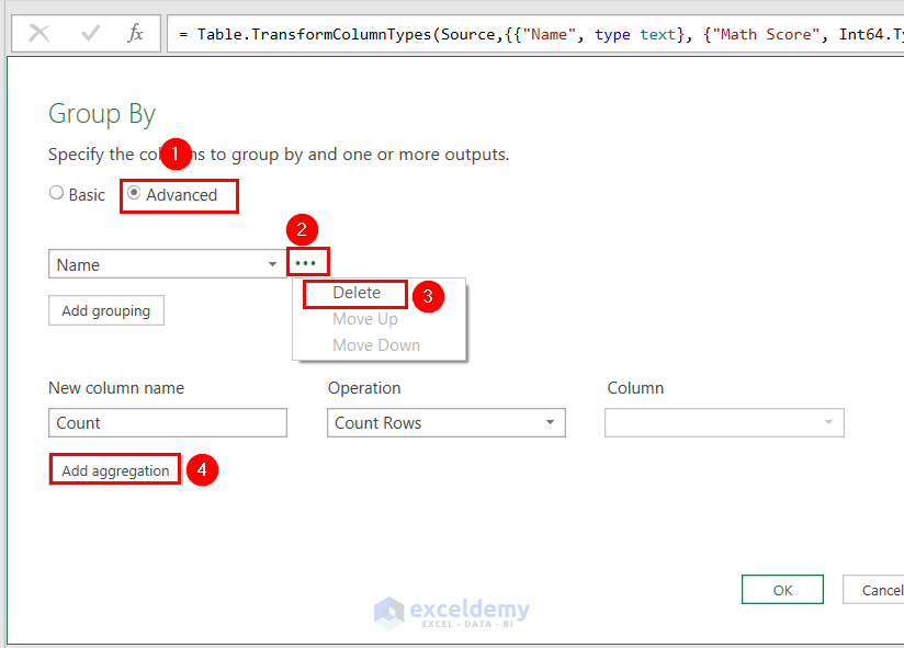
- In the Group By dialog box, select Advance.
Name box has three dots on the right side.
- Click the dots.
- Select Delete.
- Click Add aggregation to add another group.
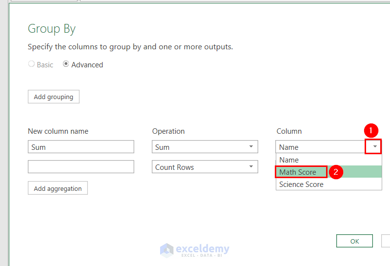
- Enter Sum in the first New column name.
- In Operation, click the drop-down arrow in Count Rows >> select Sum.
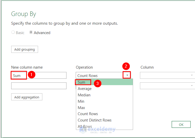
- In Column, click the drop-down arrow in Name.
- Select Math Score from the drop list.
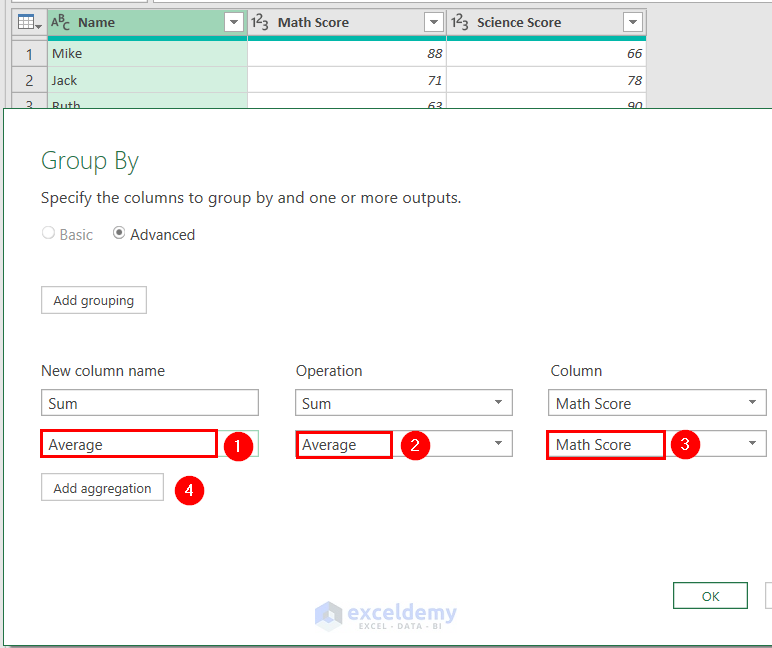
- Enter Average in the second New column name.
- Select Average in Operation.
- Select Math Score in the second Column.
- To add another group, click Add aggregation.
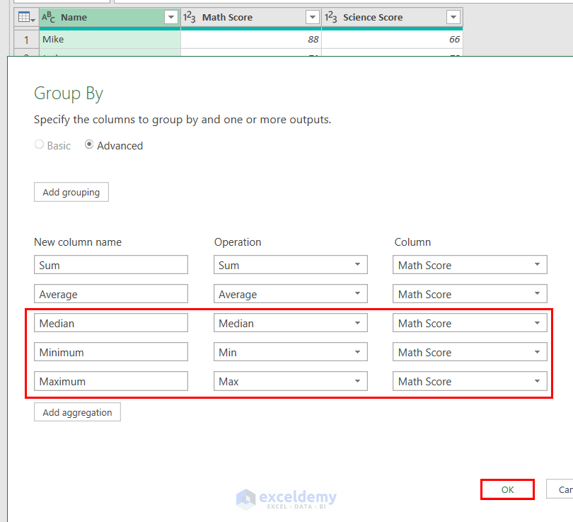
- Follow the same procedure to add 3 more groups: Median, Maximum, and Minimum.
- Click OK.
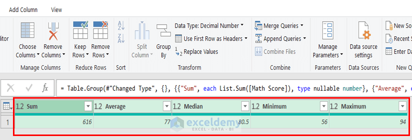
You will see the summary statistics in the Power Query.
Import the summary statistics to the Excel sheet.
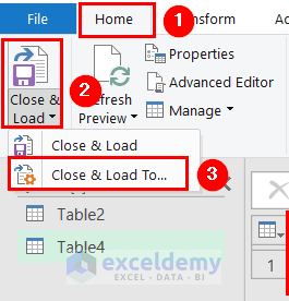
- Go to the Home tab.
- In Close & Load >> select Close & Load To.
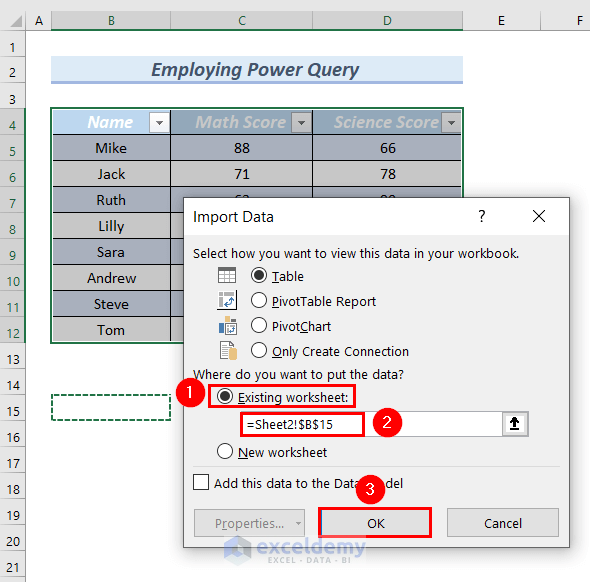
- In the Import Data dialog box, select the Existing Worksheet.
- Select B15 to enter the data.
- Click OK.
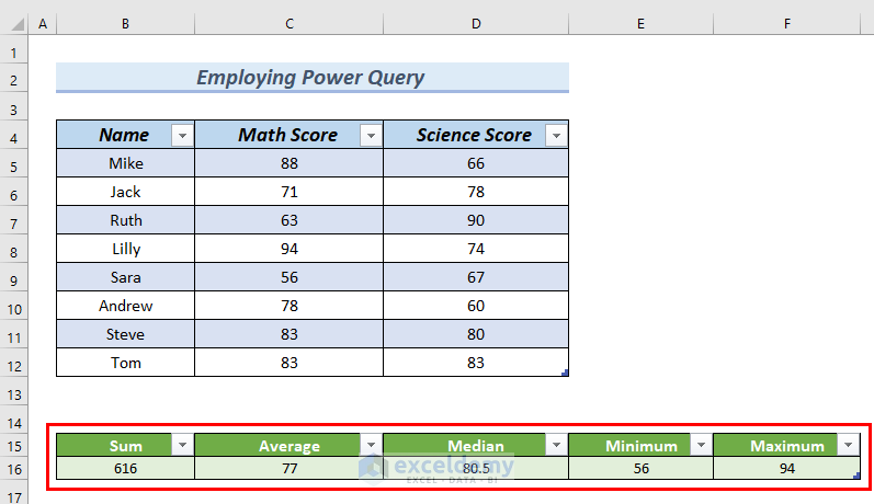
The summary statistics of the Math Score are displayed.
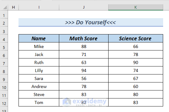
Practice Section
Download the Excel file to practice.
Download Practice Workbook
Download the Excel file and practice.
<< Go Back to Excel for Statistics | Learn Excel
Get FREE Advanced Excel Exercises with Solutions!
