Create a Functional To Do List in Excel – 4 Methods

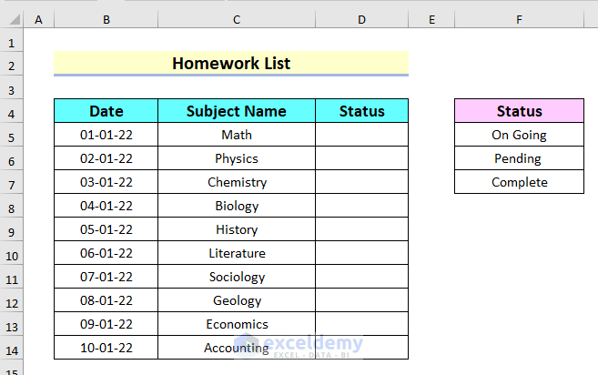
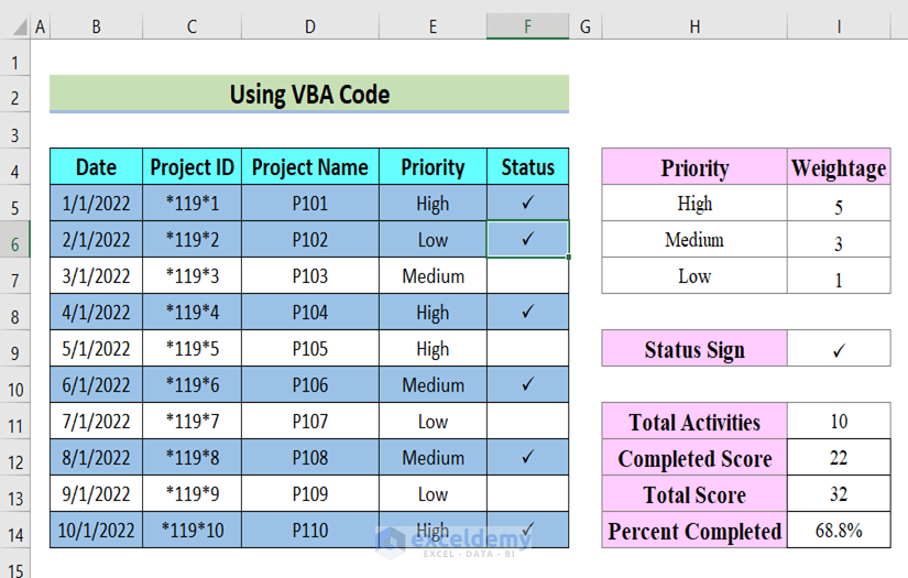
The following dataset showcases a Homework List table with Date, Subject Name, and Status.

Method 1 – Using a Drop Down List to Create a Functional To Do List

Steps:

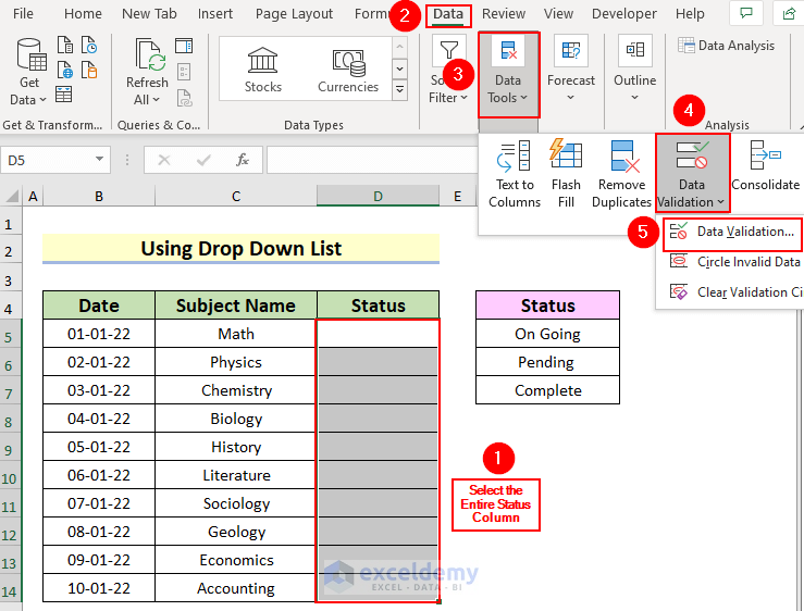
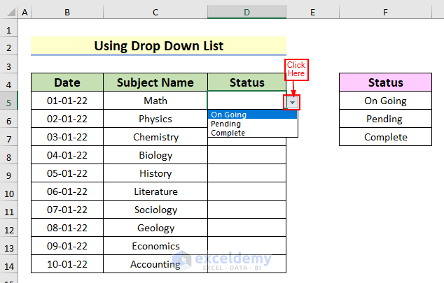
• Select the Status column:  D5:D14.
• Go to the Data tab > select Data Tools > select Data Validation > Data Validation.

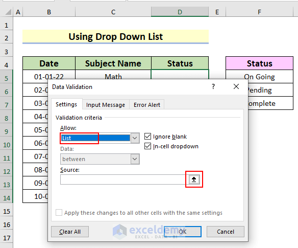
In the Data Validation dialog box:

• In Allow, select List.
• In Source, click the upward arrow marked red.

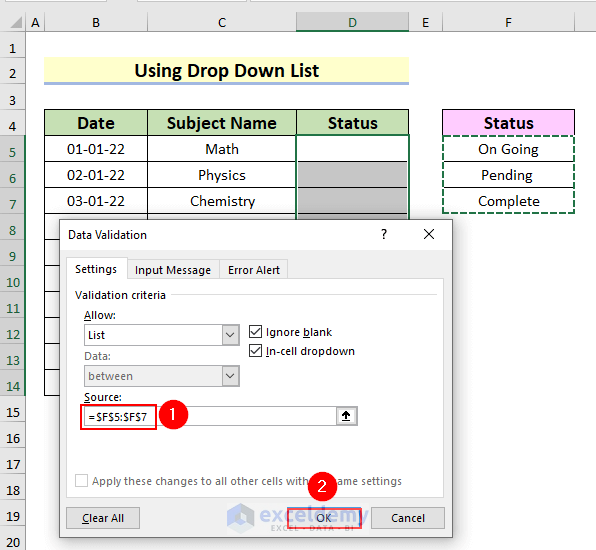
• Select F5:F7 as Source > click OK.

A down arrow is displayed at the right bottom of D5.

• Click the arrow to see the status names.
• Select On Going.

The Status is displayed in D5.

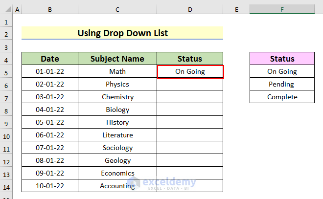
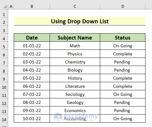
This is the output.

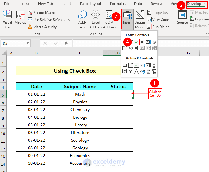
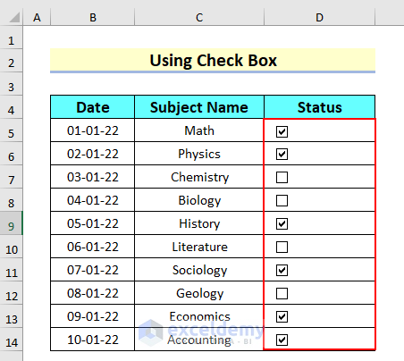
Method 2 – Using a Check Box to Create a Functional To Do List

Steps:

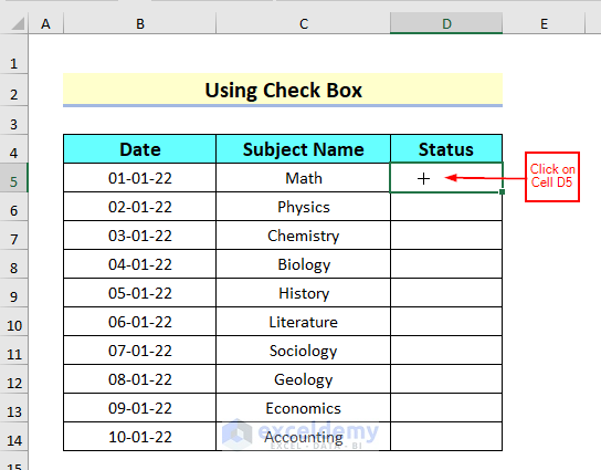
• Click a cell, here, D5 > go to the Developer tab > click Insert > select Check Box.

A plus sign is displayed in D5.

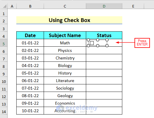
• Click D5.

You will see a Check Box in D5.

• Press ENTER.

• Drag down the Check Box using the Fill Handle tool.

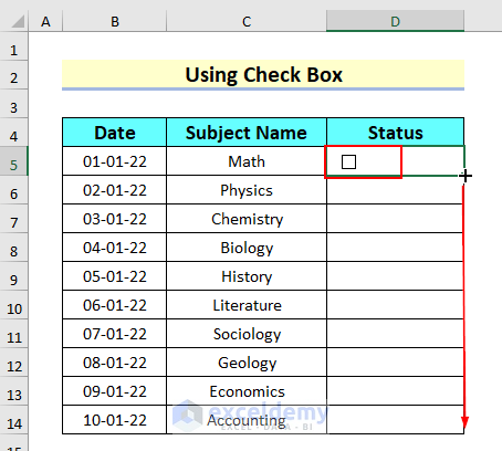
The Check Box is displayed in each cell of the Status column.

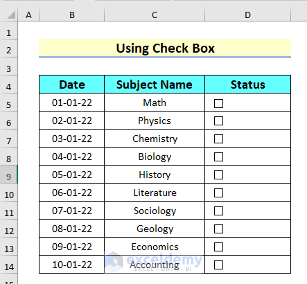
• Click the Check Box to show whether the homework is complete.

This is the output.

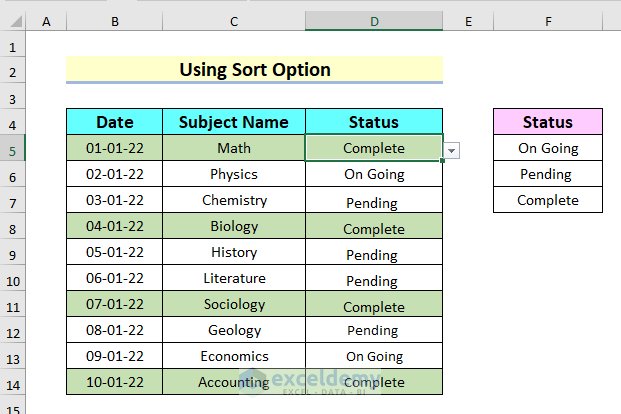
Method 3 – Using the Sort Option to Create a Functional To Do List

Steps:

• Complete the Status column by following the steps described in Method 1.

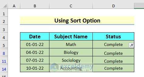
Keep the rows highlighted in green to show Complete in the Status column. Filter these rows.

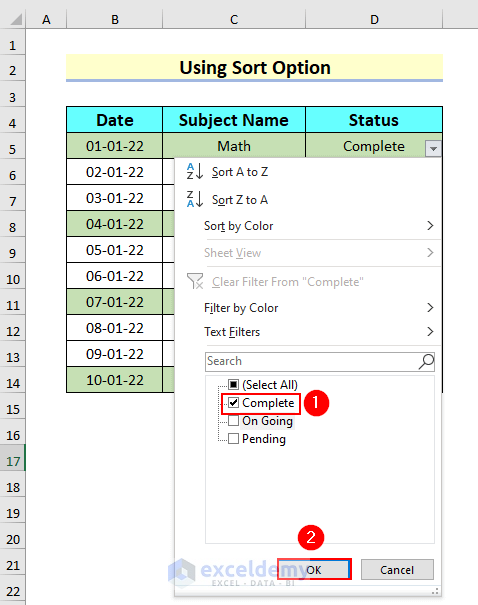
• Select the entire Status column: D5:D14 > go to the Home tab > select Editing > select Sort & Filter > select Filter.

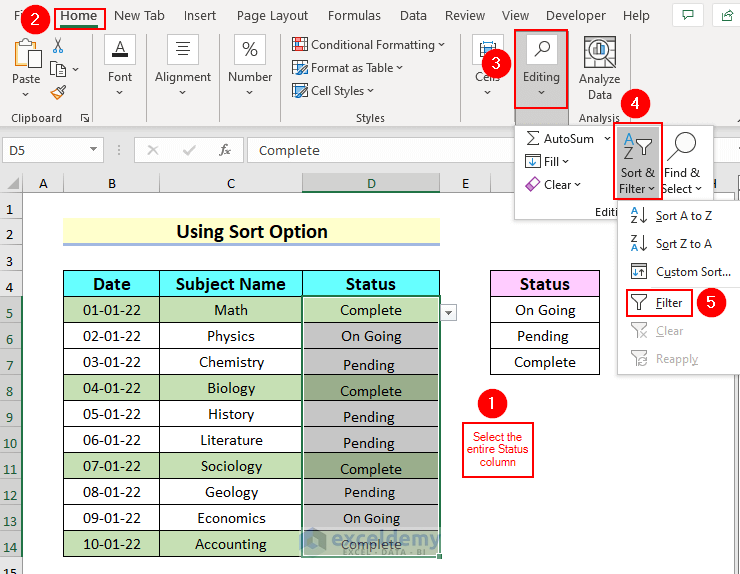
You can see a downward arrow marked red in D5.

• Click the arrow.

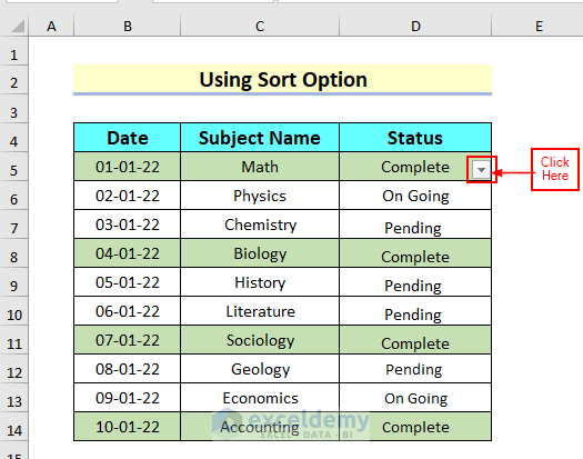
• Check Complete > click OK.

This is the output.

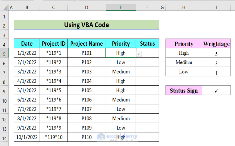
Method 4 – Using Excel an Formula and VBA to Create a Functional To Do List

Steps:

• Complete the Priority column by following the steps described in Method 1.

Here, for the Priority list, take Weightage and in G5 we insert a Status Input symbol.

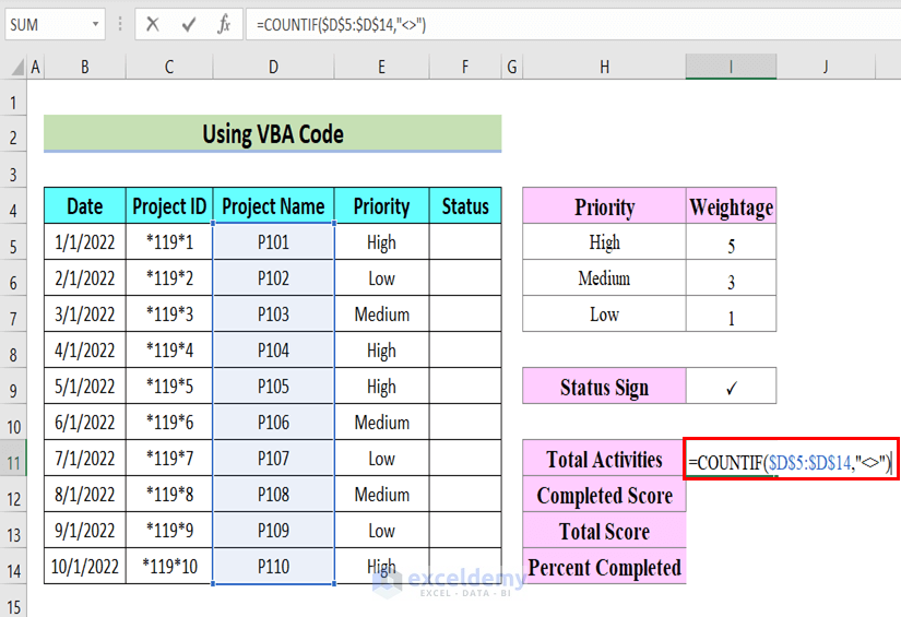
To calculate the Total Activities, Completed Score, Total Score, and %Completed, use the COUNTIF, COUNTIFS and IFERROR functions.

• Select I11 and enter the following formula to calculate the Total Activities.

• Press ENTER.

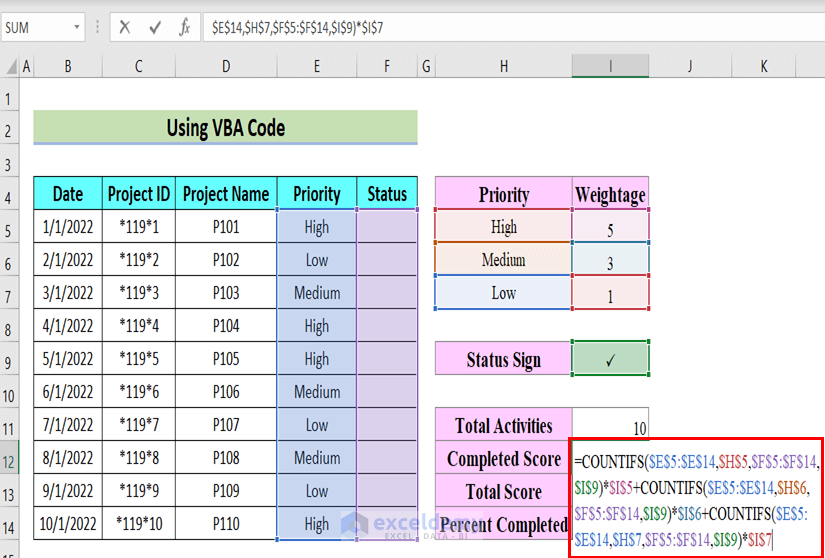
• Enter the following formula in I12 to calculate the Completed Score.

• Press ENTER.

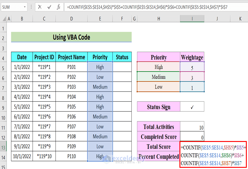
• Use the following formula in I13 to calculate the Total Score.

• Press ENTER.

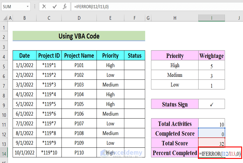
• Enter the following formula in I14 to find the Percent Completed.

• Press ENTER.

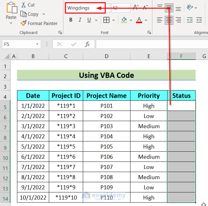
• Keep I9 in Wingdings Font.

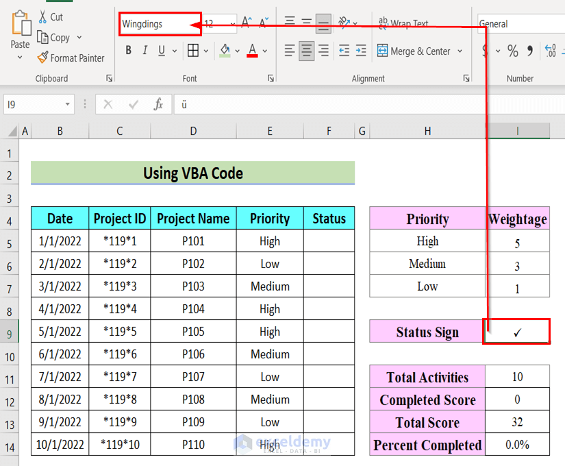
• Keep the Status column in Wingdings Font.

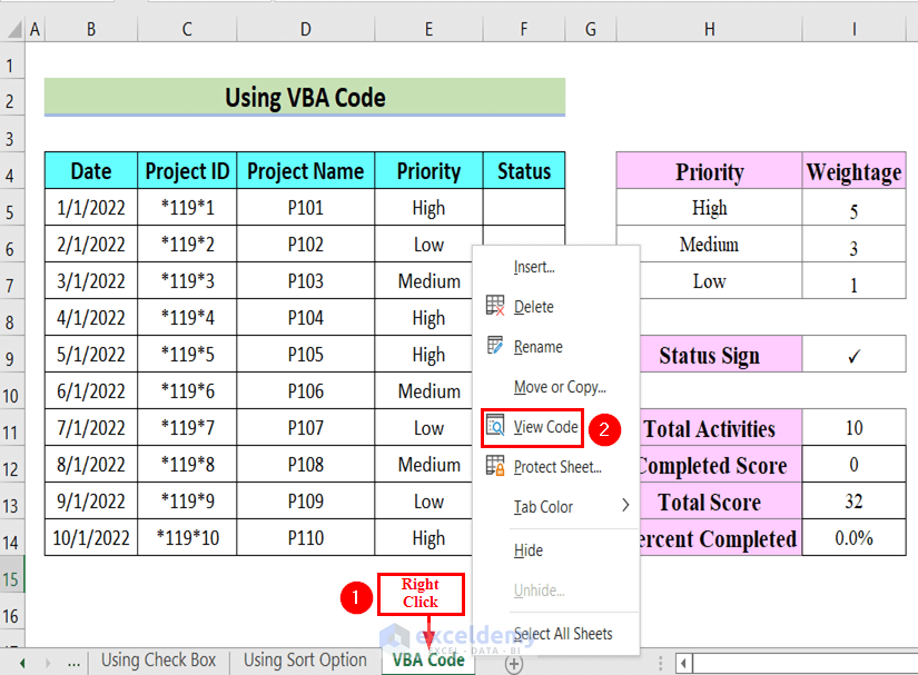
Use a VBA code to create a functional to do list.

• Right-click the VBA Code sheet > select View Code.

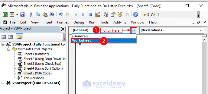
In the VBA editor window:

• Click the downward arrow in General > select Worksheet.

• Click the downward arrow in SelectionChange > select BeforeDoubleClick.

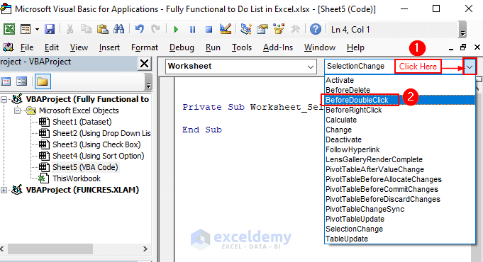
• Enter the following code in the VBA editor window.

Private Sub Worksheet_BeforeDoubleClick(ByVal Target As Range, Cancel As Boolean)
Cancel = False
    If Target.Row >= 5 And Target.Row <= 14 And Target.Column = 6 Then
    Cancel = True
        If Cells(Target.Row, Target.Column) <> Range("I9").Value Then
            Cells(Target.Row, Target.Column).Value = Range("I9").Value
        Else: Cells(Target.Row, Target.Column).Value = ""
     End If
End If
End Sub

• Close the VBA window and go back to the worksheet.
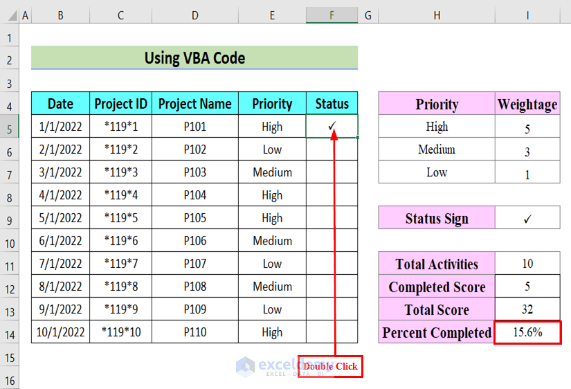
• Double-click F5.

A Check mark is displayed. 15.6% is displayed in %Completed.

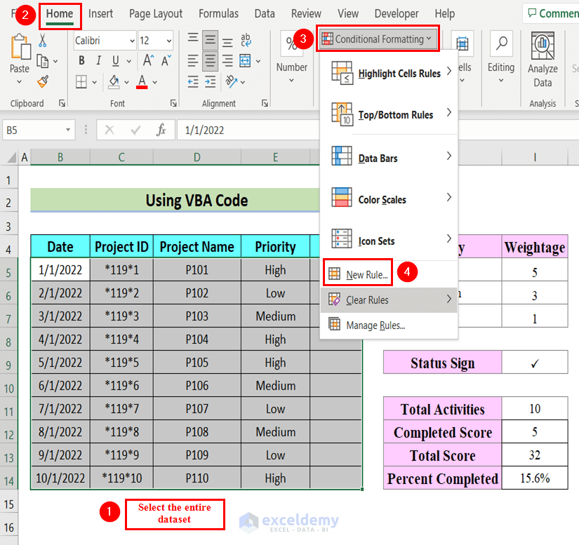
To highlight the Status row:

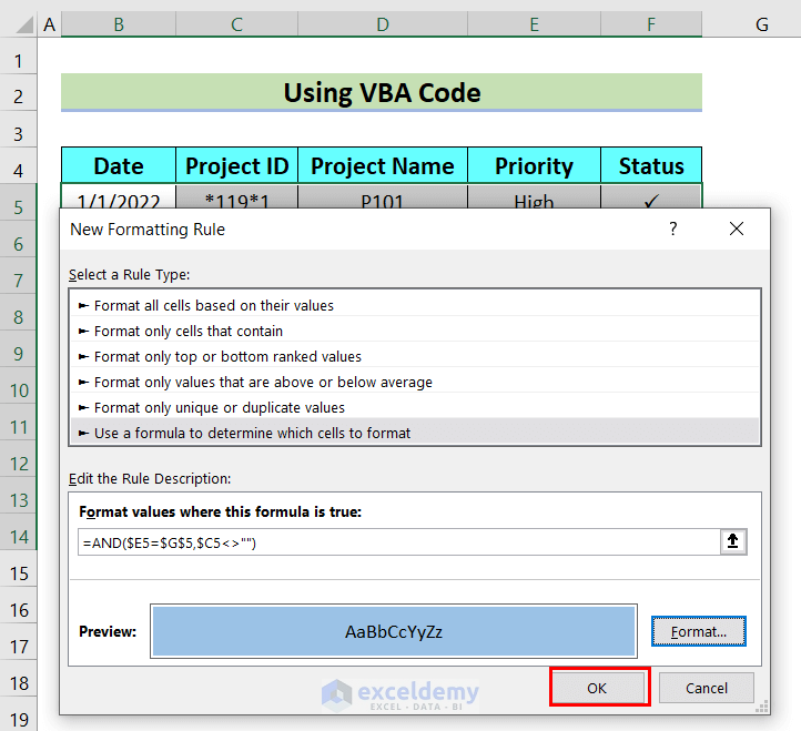
• Select the entire dataset > go to the Home tab > select Conditional Formatting > select New Rule.

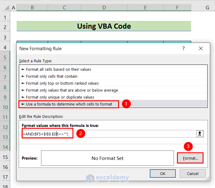
In the New Formatting Rule window:

• Select Use a formula to determine which cells to format.
• Enter the following formula in Format value where this formula is true.

• Click Format.

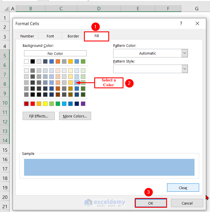
In the Format Cells window:

• Select a color. Here, blue. > click OK.

In the New Formatting Rule window, you can see the Preview.

• Click OK.

If you double click a cell in the Status column,  you will see the entire row highlighted in blue. you will also see the %Completed in H12.

• Double click different cells to see the functional to do list.

Download Workbook

Related Articles

• Excel To Do List with Progress Tracker
• How to Make To Do List in Excel with Checkbox

<< Go Back to To-Do List in Excel | Tracker in Excel | Excel Templates