How to Put Excel Tabs on Top of Worksheet (2 Easy Ways)

The default setting in Excel positions the sheet tabs at the bottom of the workbook window. However, users may find it more convenient or visually appealing to have the tabs on top of the worksheet, resembling a setup similar to popular web browsers. This arrangement allows for easier navigation between sheets, especially when working with a large number of worksheets within a workbook.

In this Excel tutorial, you will learn how to put tabs on top of a worksheet using VBA code and adding hyperlinks.

In the GIF below, you can see how to access worksheets from the Quick Access Toolbar (QAT) which are added in QAT using VBA codes.

Here are 2 methods to put the Excel tabs on top of worksheets:

Using VBA to Put Excel Tabs on Top of Worksheet

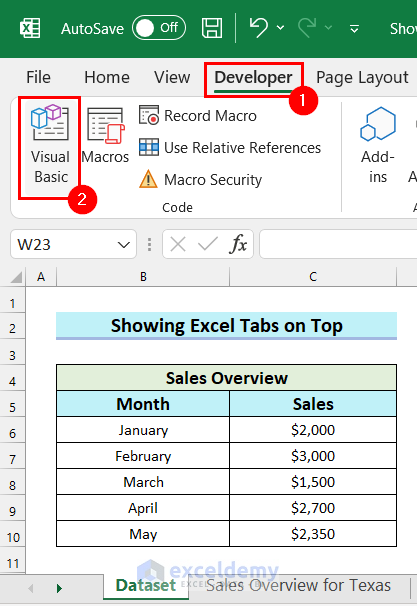
If you want to automate the process of placing tabs on top of a worksheet in Excel, you can use VBA code. This code creates a list of worksheet tabs on the Quick Access Toolbar (QAT), which is located at the top of your worksheet. By accessing the tabs from the QAT, you can quickly navigate between them.

To place Excel tabs on top of the worksheet using VBA code, follow the steps below:

Go to the Developer tab > Code group > Visual Basic. Or, press ALT + F11.
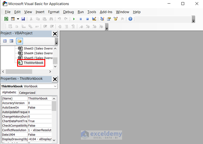
In the Visual Basic window, select ThisWorkbook from VBAProject.

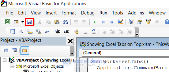
Write the following code in the ThisWorkbook module.

Sub WorksheetTabs()
  Application.CommandBars("Workbook tabs").ShowPopup
End Sub

Save the code and go back to your worksheet.
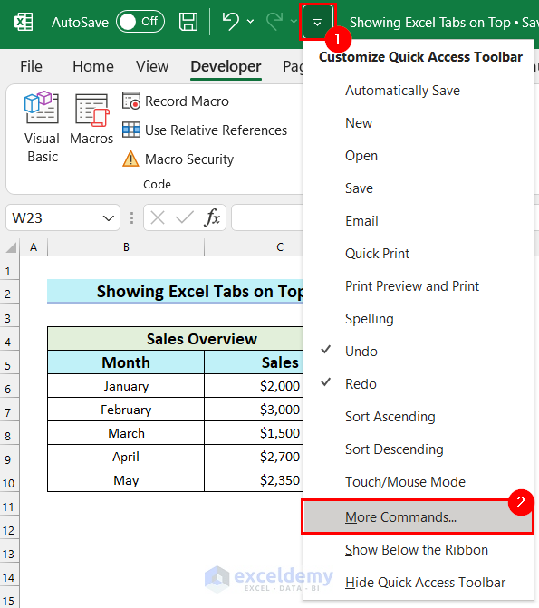
Select the drop-down icon for the Quick Access Toolbar.
Select More Commands.
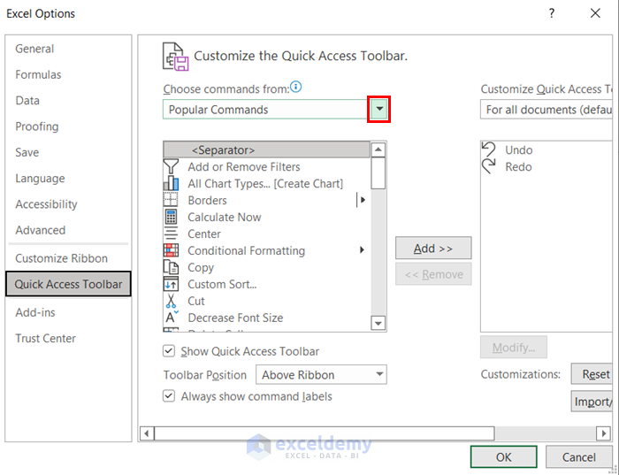
In the Excel Options dialog box, click on the drop-down option of “Choose commands from”.
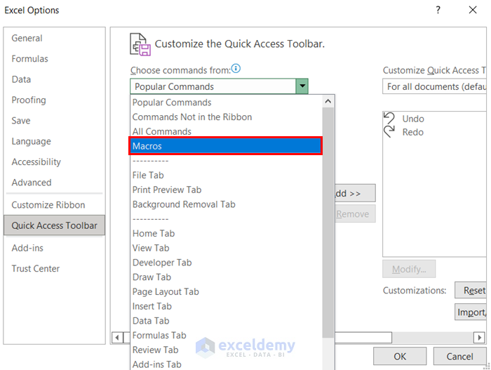
Select Macros from the options.
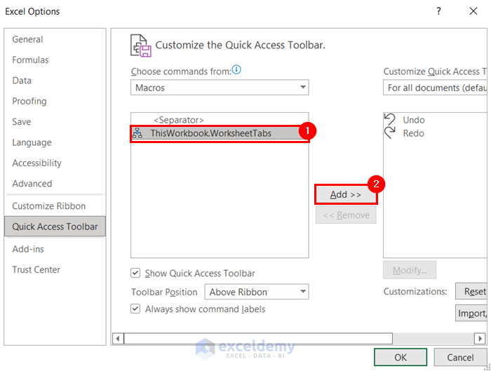
Select the macro, click on Add, and press OK.

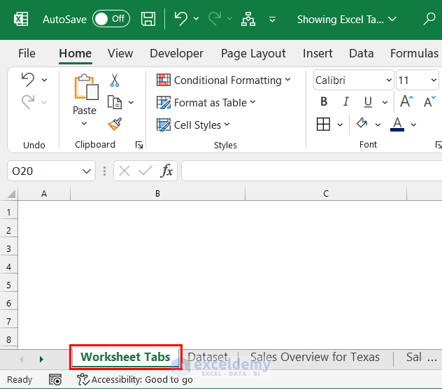
In the following GIF, you can see the list of Excel tabs on top of the worksheet. You can go to any worksheet directly by using this list. To do that, just select the worksheet you want to go. Here, I selected the sheet named Sales Overview for Virginia. You can see that the sheet named Sales Overview for Virginia is open.

Note:

When working with macros in Excel, you must save the workbook as an Excel Macro-Enabled Workbook.

Applying HYPERLINK Function to Put Excel Tabs on Top of Worksheet

In this method, you will learn to add a hyperlink using the HYPERLINK function to put Excel tabs on top of the worksheet. The HYPERLINK function brings out a cutoff link that will open on a server, or make a move to other worksheets. Excel opens the URL when we click the cell that holds the HYPERLINK function.

Follow the steps below to put Excel tabs on top of the worksheet using the HYPERLINK function:

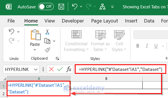
Create and name a new worksheet to put all the worksheet tabs.
Here, we created a worksheet named Worksheet Tabs.
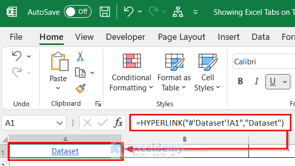
Write the following formula in cell A1: =HYPERLINK("#'Dataset'!A1","Dataset")
Here, in the HYPERLINK function, I selected “#’Dataset’!A1” as “link_location”, and “Dataset” as “friendly_name” argument. The function will return a link that will directly lead to the selected location, which is cell A1 of the sheet named “Dataset”.
Press ENTER to get the result.

Similarly, you can add hyperlinks to other worksheets. Such as in cell B1, insert the following formula: =HYPERLINK("#'Sales Overview for Texas'!A1","Sales Overview for Texas")

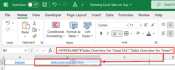
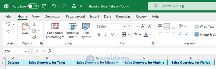
Thus you can see the “Sales Overview for Texas” tab is hyperlinked in cell B1.

Following this method, we have inserted all the other worksheet links. You can see the Excel tabs on the top row of the worksheet. To make these links more eye-catching, format the cells according to your choice. We formatted them with fill color and bold font.

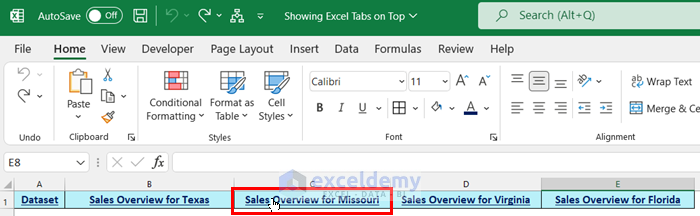
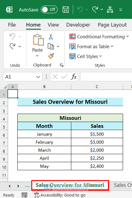
Now, you can go to any worksheet from this worksheet directly by using these links. Just select the worksheet you want to go to. Here, I selected the sheet named Sales Overview for Missouri.

You can see that the sheet named Sales Overview for Missouri is open.

Download Practice Workbook

Showing Excel Tabs on Top.xlsm

Conclusion

In this Excel tutorial, you have learned two easy methods to put Excel tabs on top of a worksheet. One method uses VBA to add the sheets in the Quick Access Toolbar for better navigation to tabs. The other method uses the hyperlinking method. This method makes the tabs appear on the top row of your sheet for better visualization. If you have any questions, please let me know in the comment section.

Frequently Asked Questions

Why is Excel not showing tabs?

The “Show sheet tabs” feature might be disabled. To enable it, follow these steps:

Click on File > Options > Advanced.
Under “Display options for this workbook“, make sure that the “Show sheet tabs” box is checked.

Can I change the order of sheet tabs in Excel?

Yes. The easiest way to change the order of sheet tabs is to select and drag them to the location you want to place them.

Is it possible to group or color-code Excel sheet tabs?

Yes. To group or color-code Excel sheet tabs, right-click on the tab, select Tab Color from the context menu, and choose a color.

<< Go Back to Sheets Tab in Excel | Excel Parts | Learn Excel

Get FREE Advanced Excel Exercises with Solutions!