Microsoft Excel presents various sort options. Sorting may differ in terms of our needs and conditions. What we need to know is the correct and proper use of the sorting options in Excel. Sorting dates may help us to manage our data more effectively and efficiently. In this article, we will see 6 effective ways to sort dates in chronological order in Excel. I hope it will be very helpful for you if you are looking for a simple and easy, yet effective way to sort dates in chronological order in Excel.
How to Sort Dates in Chronological Order in Excel (6 Effective Ways)
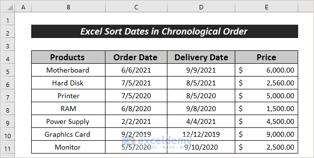
In order to sort dates in chronological order in Excel, there are many simple and effective ways. I am going to discuss 6 of them here. For more clarification, I am going to use a dataset where I have arranged data in the Products, Order Date, Delivery Date, and Price columns.
1. Adopt Sort & Filter Option
Adopting the Sort & Filter option is the simplest way to sort dates in chronological order. The whole process is described in the following section.
Steps:
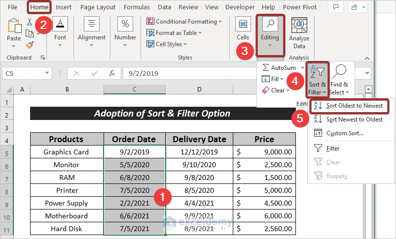
- Select the dates that you want to sort in chronological order.
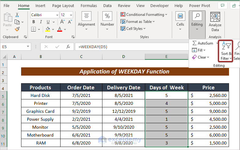
- Next, go to the Home tab.
- From the ribbon, select Editing along with Sort & Filter.
- Now, choose your sorting pattern from the available options. I have picked Sort Oldest to Newest.
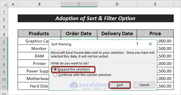
A warning box will appear.
- Mark the box having Expand the selection.
- Finally, click on Sort.
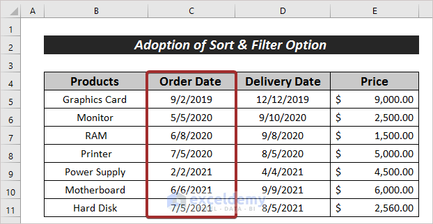
Now, we can see the sorted dates in chronological order on the selected cells.
Read More: How to Sort by Date in Excel
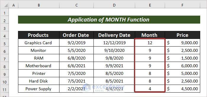
2. Apply MONTH Function
The MONTH Function can be another quick way to sort dates in chronological order. It helps to find the number of the month in the year. We can then use it to sort dates in chronological order.
Steps:
- Select a cell and input the following formula to have the month number.
=MONTH(D5)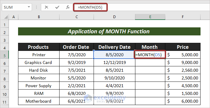
- Next, press ENTER to have the output.
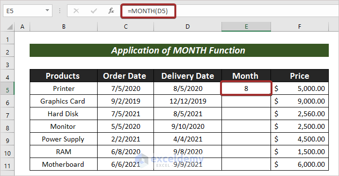
- Now, use Fill Handle to AutoFill the rest cells.
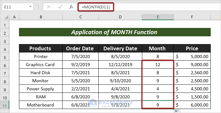
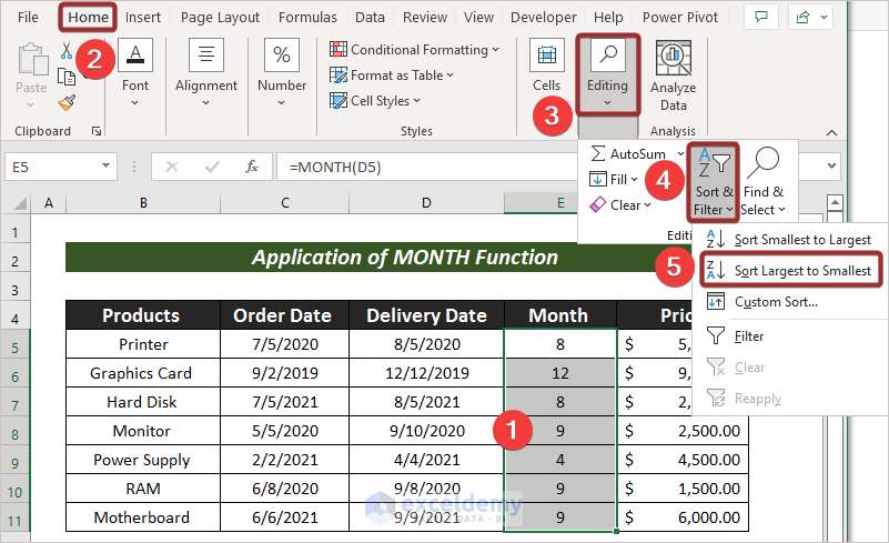
- After that, go to the Home tab.
- From the ribbon, select Editing along with Sort & Filter.
- Now, choose your sorting pattern from the available options. I have picked Sort Largest to Smallest.
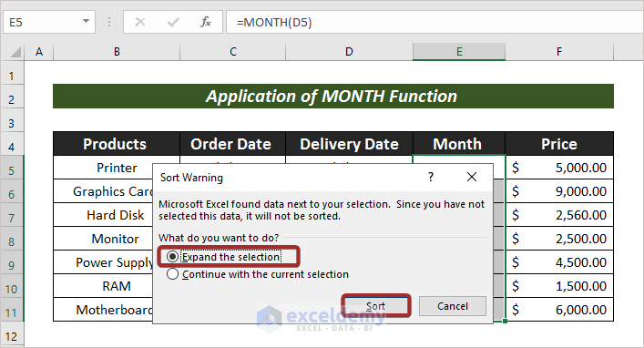
A warning box will appear.
- Followingly, Mark the box having to Expand the selection.
- Finally, click on Sort.
Thus, we can have the sorted dates in chronological order on the selected cells.
Read More: How to Sort Dates in Excel by Year
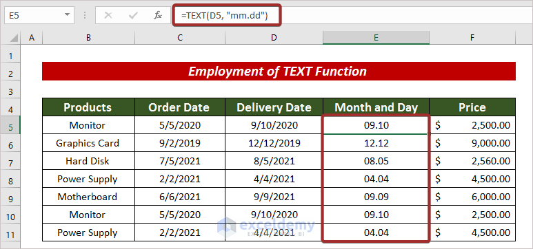
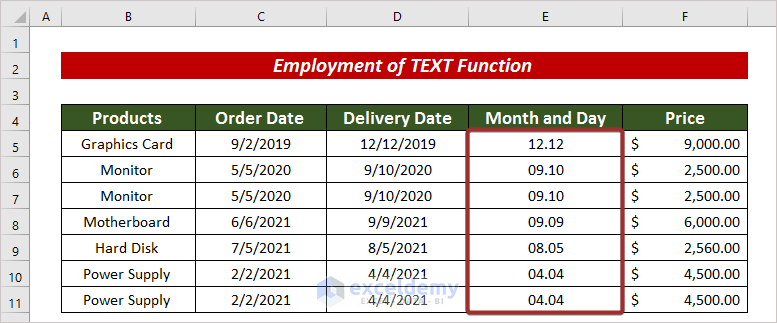
3. Employ TEXT Function
In order to sort the dates in chronological order, we can also consider month and day. For this, the required functions are MONTH and DAY. And again, our dataset will be the same as the previous one and the additional column will be named Month and Day.
Steps:
- First of all, create a column (i.e. Month and Day) and input the following formula to have month and day values.
=TEXT(D5, "mm.dd")- Press ENTER and AutoFill the rest cells.
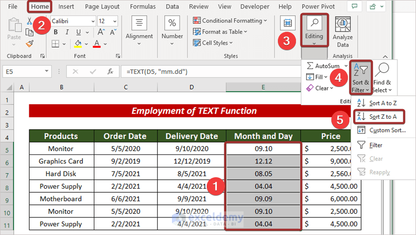
- Afterward, click on Home.
- Go to Editing along with Sort & Filter from the ribbon.
- Now, choose your sorting pattern from the available options. I have picked Sort Z to A.
We can see our desired output on the screen.
4. Use YEAR Function
The YEAR Function is used to find the year from a date. We can also sort dates in chronological order based on year.
Steps:
- Use the following formula to have the year values.
=YEAR(D5)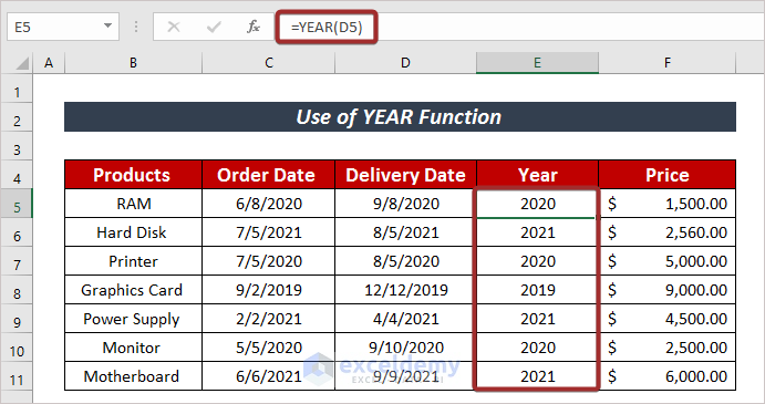
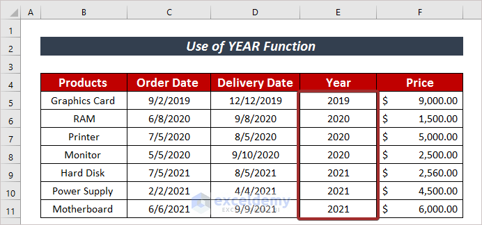
- Then, use Sort & Filter under the Home tab to sort dates according to your preferred chronological order.
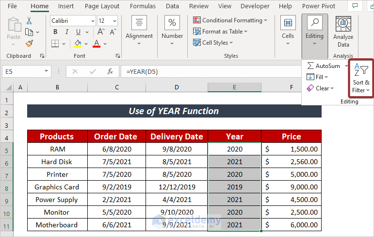
I have used the Sort Smallest to Largest order to sort dates.
Read More: How to Sort Dates in Excel by Month and Year
5. Apply WEEKDAY Function
Another very easy way to sort dates in chronological order is to use the WEEKDAY function. The WEEKDAY Function is used to find the day’s number of a week. We can also sort dates in chronological order based on that.
Steps:
- Input the following formula to have the day’s number of a week.
=WEEKDAY(D5)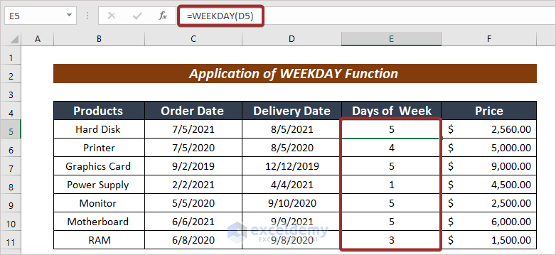
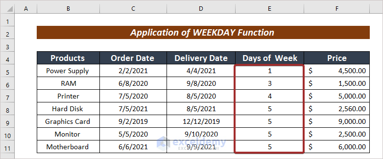
- After that, click on Sort & Filter under the Home tab to sort dates according to your preferred chronological order.
In this case, I have used the Sort Smallest to Largest order to sort dates.
6. Combine IFERROR, INDEX, MATCH, COUNTIF & ROWS Functions
Adopting a combined formula with the IFERROR, INDEX, MATCH, COUNTIF, and ROWS functions, we can also sort dates in chronological order.
Steps:
- Select a cell and input the following formula in that cell.
=IFERROR(INDEX($D$5:$D$11, MATCH(ROWS($D$10:D10), COUNTIF($D$5:$D$11, "<="&$D$5:$D$11), 0)), "")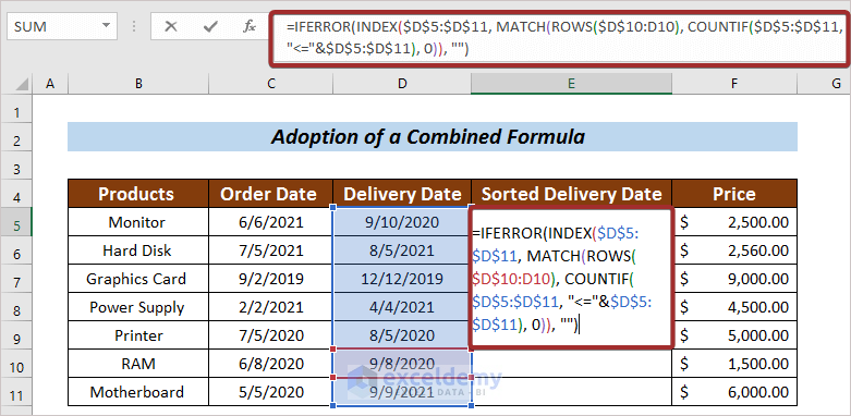
- Next, press on ENTER.
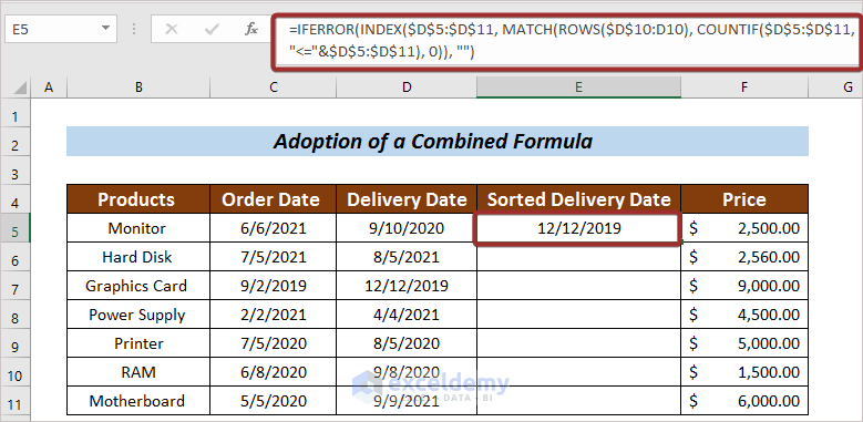
We can see the oldest date in that cell.
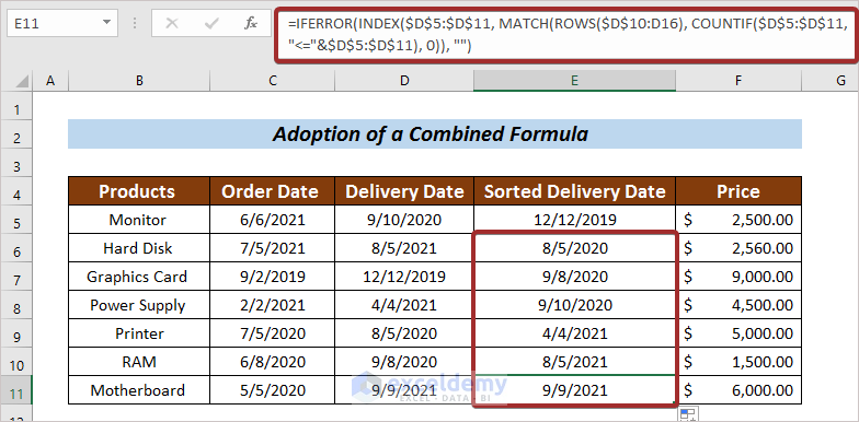
- Finally, AutoFill the remaining cells.
Read More: How to Sort by Date and Time in Excel
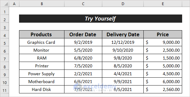
Practice Section
You can practice in the following section for more expertise.
Download the Practice Workbook
Conclusion
At the end of this article, I like to add that I have tried to explain 6 effective ways to sort dates in chronological order in Excel. It will be a matter of great pleasure for me if this article could help any Excel user even a little. For any further queries, comment below. You can visit our site for more articles about using Excel.
Related Articles
<< Go Back to Sort by Date in Excel | Sort in Excel | Learn Excel
Get FREE Advanced Excel Exercises with Solutions!

Sorting the dates using your 6th method with the IFERROR, INDEX, MATCH, COUNTIF & ROWS Functions is intriguing. However I don’t understand why, in your example, the Rows function starts at D10. The column for that table starts at D5 and ends at D11.
Can you explain your 6th method in alot more detail please? Will this work in Excel versions that are earlier than 365? Will it also sort dates generated by formula in a dynamic table, ie there are empty rows as well.
Hello CJ,
Thanks for your comment. To go into the details of your queries, let me break down the formula for you used in method 6 in a simpler form first.
The whole formula was:
=IFERROR(INDEX($D$5:$D$11, MATCH(ROWS($D$10:D10), COUNTIF($D$5:$D$11, “<=”&$D$5:$D$11), 0)), “”)
Here, the ROWS function counts the number of rows in the defined array.
ROWS($D$10:D10) → 1
The COUNTIF function compares the values in the given range and denotes them with a number based on the position in the smallest to largest order.
COUNTIF($D$5:$D$11, “<=”&$D$5:$D$11) → {4;6;1;5;2;3;7}
The MATCH function compares the values returned by the ROWS & COUNTIF functions and returns the index number of the position of the exact match.
MATCH(1, COUNTIF($D$5:$D$11, “<=”&$D$5:$D$11), 0))
MATCH(1, {4;6;1;5;2;3;7})→ 3
The INDEX function returns the third date value from the defined range in general form.
INDEX($D$5:$D$11, MATCH(ROWS($D$10:D10), COUNTIF($D$5:$D$11, “<=”&$D$5:$D$11), 0))
INDEX($D$5:$D$11, 3) → 43811
If there is an error in finding a date, the IFERROR function will return a blank cell as an output.
While applying the ROWS function, I have set a reference point from D10 and also finished the array on D10. That returns the number of row count 1. However, it is not mandatory that you have to set the reference point from D10. You can start from any cell between D5 to D11 but the starting and ending cell reference should be the same in that array. You can apply “ROWS($D$5:D5)” and it will return 1 too which is the same output.
If I am not wrong, the IFERROR function was introduced in the 2007 Excel version and the INDEX, MATCH, COUNTIF, & ROWS functions are available in the earliest Excel versions too. So, I hope it will work perfectly from the 2007 and the later Excel versions.
This formula can be applied to a dynamic table. It will automatically sort dates within the given range.
I hope you have the answers that you were looking for.
Regards,
Naimul Hasan Arif