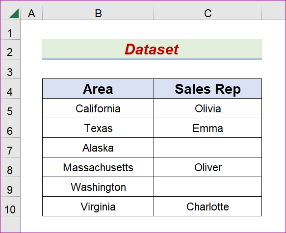
The following dataset consists of two columns labeled Area and Sales Rep. It has several records that are missing important information. We are going to utilize each of the three methods to return the cells that have data from a range, and then we are going to collect that data in a new column that is going to be called Sales Rep List.
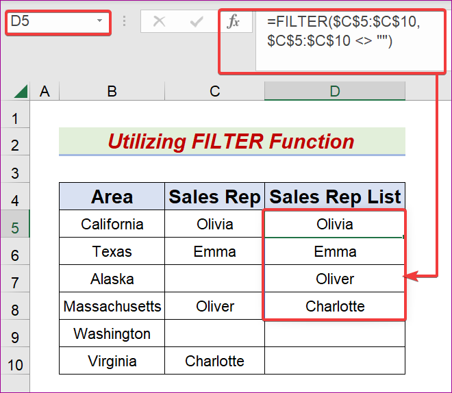
Method 1 – Utilize the FILTER Function to Display Non-Blank Cells from a Field in Excel
Steps:
- Create another column D titled Sales Rep List.
- Select the D5 cell.
- Copy the following formula in the Formula Bar.
=FILTER($C$5:$C$10,$C$5:$C$10 <> "")
- Hit the Enter or Tab key.
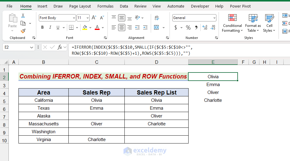
Method 2 – Combine IFERROR, INDEX, SMALL, and ROW Functions to Get Non-Empty Cells from a Range
Steps:
- Make another column D called Sales Rep List.
- Choose the D5 cell.
- Copy the following formula in the cell.
=IFERROR(INDEX($C$5:$C$10,SMALL(IF($C$5:$C$10<>"",ROW($C$5:$C$10)-ROW($C$5)+1),ROWS($C$5:$C5))),"")
- Hit Enter or Tab.
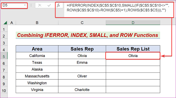
- We will get the intended outcome for D5.
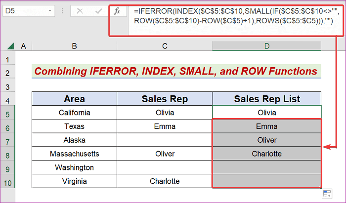
- Use the AutoFill Handle icon and drag it into cell D10.
How Does the Formula Work?
=IFERROR(INDEX($C$5:$C$10,SMALL(IF($C$5:$C$10<>””,ROW($C$5:$C$10)-ROW($C$5)+1),ROWS($C$5:$C5))),””)
For this formula to make sense, you need to know how to use the following Excel functions:
IFERROR, INDEX, SMALL, ROW and Rows Functions
- ROW($C$5:$C$10)-ROW($C$5)+1)
The ROW function within Excel provides the cell’s row number. By involving the Row function in the combination, we find- {1;2;3;4;5;6}.
- IF($C$5:$C$10<>””,ROW($C$5:$C$10)-ROW($C$5)+1)
Checks which cells in the range are not blank. For every non-blank cell, it returns the relative row position inside the range. For blank cells, it returns FALSE
- ROWS($C$5:$C5))
The ROWS function will retrieve the total number of rows included when passing an Excel range. In this demo, it will produce 1 for the first row.
- SMALL(IF($C$5:$C$10<>””,ROW($C$5:$C$10)-ROW($C$5)+1),ROWS($C$5:$C5))
The SMALL function provides ranked numerical values according to their location in a given list. It finds the k-smallest item in a particular dataset and delivers the deals. The SMALL function produces 1 as an outcome for the first row.
- INDEX($C$5:$C$10,SMALL(IF($C$5:$C$10<>””,ROW($C$5:$C$10)-ROW($C$5)+1),ROWS($C$5:$C5)))
To get data from a specific location in a column or range, use the INDEX function. Olivia will appear at the top of the list in this case.
- IFERROR(INDEX($C$5:$C$10,SMALL(IF($C$5:$C$10<>””,ROW($C$5:$C$10)-ROW($C$5)+1),ROWS($C$5:$C5))),””)
The IFERROR is a function that tells whether the cells or formulas contain calculation mistakes. We will get Errors when we try to work with empty cells, and we will use the IFERROR function to avoid these errors.
Method 3 – Run Excel VBA Code to Return Non-Blank Cells from a Range
Steps:
- Choose the intended sheet as the Active sheet.
- Create another column D.
- Navigate to the Developer tab and click the Visual Basic icon.

- Click on Insert and Module
![]()
- Input the following code in the Module box.
Sub ReturnNonBlankCells()
    Range("D5").Select
    ActiveCell.Formula2R1C1 = "=FILTER(R5C3:R10C3," & Chr(10) & "R5C3:R10C3 <> """")"
End Sub- Press F5 or the Save button.
![]()
- This will provide the desired result like the one below.
![]()
Read More: Formula to Return Blank Cell instead of Zero in Excel
Download the Practice Workbook
Related Articles
- How to Find Blank Cells in Excel
- Null vs Blank in Excel
- How to Highlight Blank Cells in Excel
- How to Set Cell to Blank in Formula in Excel
- How to Make Empty Cells Blank in Excel
- How to Deal with Blank Cells That Are Not Really Blank in Excel
<< Go Back to Excel Cells | Learn Excel
Get FREE Advanced Excel Exercises with Solutions!

Basically Method 2 doesn’t work and is incorrectly shown as
=IFERROR(INDEX($C$5:$C$10,SMALL(IF($C$5:$C$10″”,ROW($C$5:$C$10)-ROW($C$5)+1),ROWS($C$5:$C5))),””)
Also notes at the bottom says ISERROR
As shown the formula will only work for the first row.
Same wrong example has been around decades.
AI also replies with the same wrong example because of articles like this.
Hello Clive Emberey,
Thank you for your detailed feedback. We reviewed and tested Method 2 again. The formula works correctly when the output starts in the intended first output cell. However, we understand that the ROWS($C$5:$C5) counter can be confusing if readers place the formula in a different row without adjusting the reference. We have updated the explanation to make this clearer. You were also right that the note should refer to IFERROR, not ISERROR, and we have corrected that. Thanks again for helping us improve the article.
Regards,
ExcelDemy