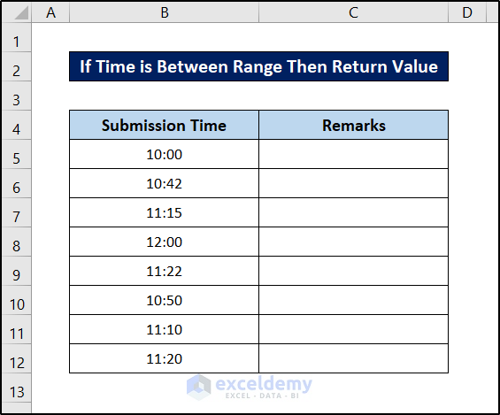
This is the sample dataset.
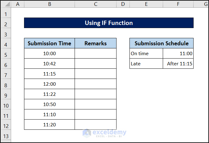
Example 1- Using the IF Function
Consider the following criteria:
Steps:
- Select a cell to see the result. Here, C5.
- Enter the following formula.
=IF(B5<=$F$5,$E$5,$E$6)
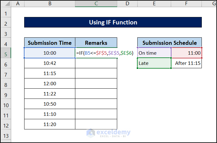
- Press Enter.
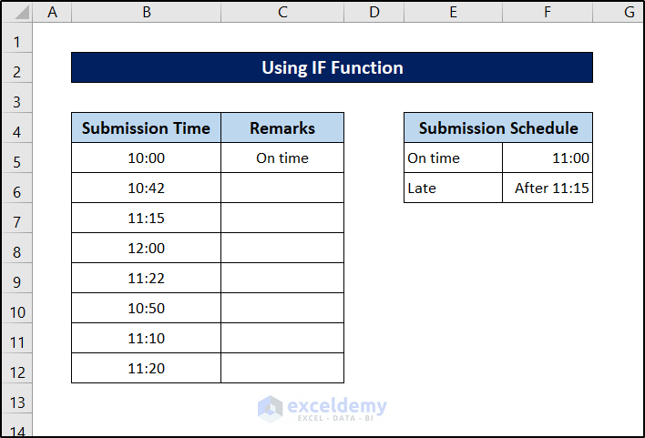
- Drag down the Fill Handle to see the result in the rest of the cells.

This is the output.
Example 2 – Utilizing Nested IF Functions

Steps:
- Select a cell to see the result. Here, C5.
- Enter the following formula.
=IF(B5<=$F$5,$E$5,IF(B5<=$F$6,$E$6,$E$7))
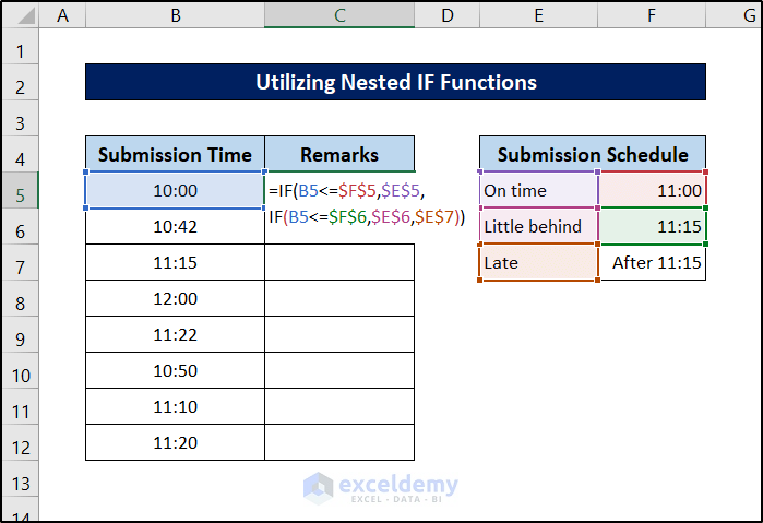
- Press Enter.

- Drag down the Fill Handle to see the result in the rest of the cells.
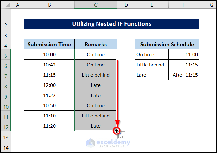
This is the output.
Formula Breakdown
IF(B5<=$F$5,$E$5,IF(B5<=$F$6,$E$6,$E$7))
IF(B5<=$F$5,$E$5,…) checks whether the value of B5 is smaller than or equal to F5. If it is smaller, it returns the value of E5. Otherwise, it moves to the next portion of the formula.
IF(B5<=$F$6,$E$6,$E$7) checks whether the value of B5 is smaller than or equal to F6. If it is smaller, it returns the value of cell E6. Otherwise, it returns the value of E7.
The first formula returns TRUE: “On time” is the value of E5.
Example 3 – Applying IFS Function
Steps:
- Select a cell to see the result. Here, C5.
- Enter the following formula.
=IFS(B5<=$F$5,$E$5,B5<=$F$6,$E$6,TRUE,$E$7)
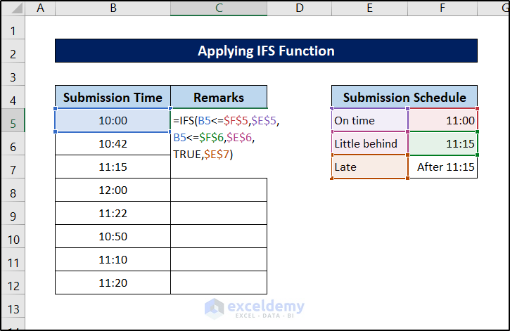
- Press Enter.
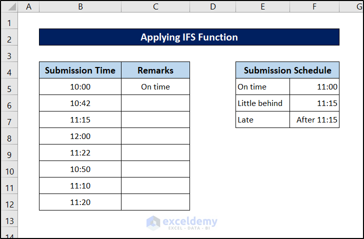
- Drag down the Fill Handle to see the result in the rest of the cells.
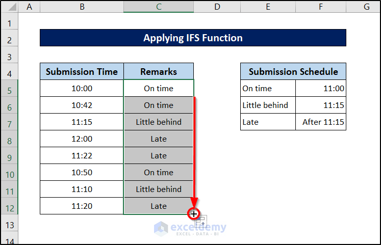
This is the output.
Example 4 – Combining the IF and the AND Functions
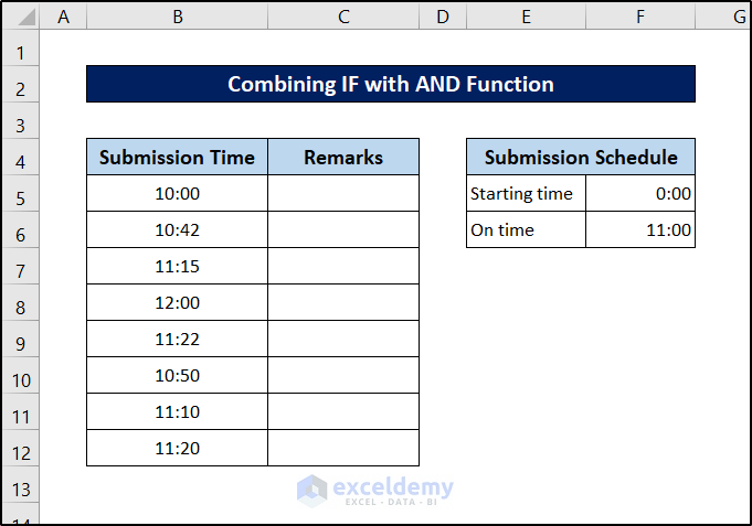
Steps:
- Select a cell to see the result. Here, C5.
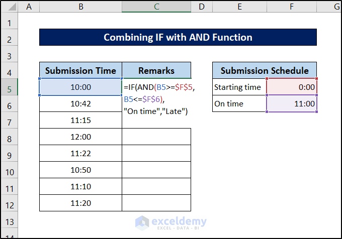
- Enter the following formula.
=IF(AND(B5>=$F$5,B5<=$F$6),"On time","Late")
Formula Breakdown
IF(AND(B5>=$F$5,B5<=$F$6),”On time”,”Late”)
There are two conditions in AND(B5>=$F$5,B5<=$F$6). The first one checks whether the value of B5 is greater than or equal to F5. The second checks whether the same value is smaller than or equal to F6. If both conditions are true, it returns TRUE. Otherwise, it returns FALSE.
IF(AND(B5>=$F$5,B5<=$F$6),”On time”,”Late”) returns “On time” if both conditions in the AND function are true. Otherwise, it returns “Late”.
- Press Enter.
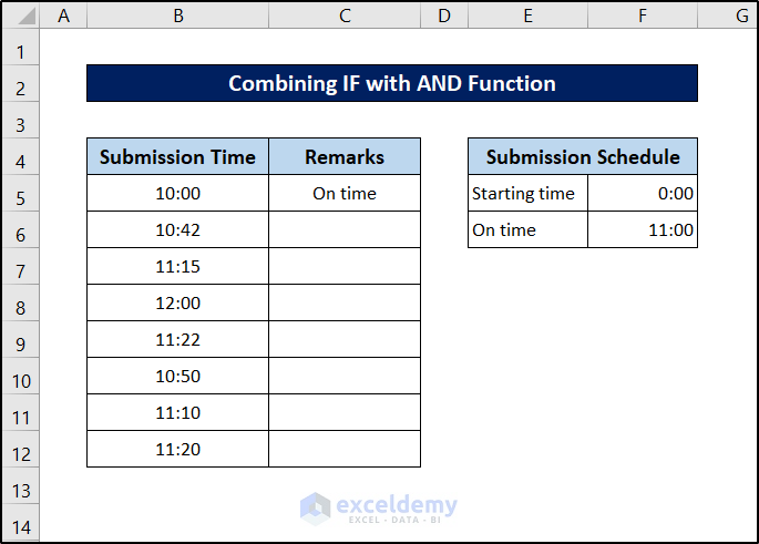
- Drag down the Fill Handle to see the result in the rest of the cells.
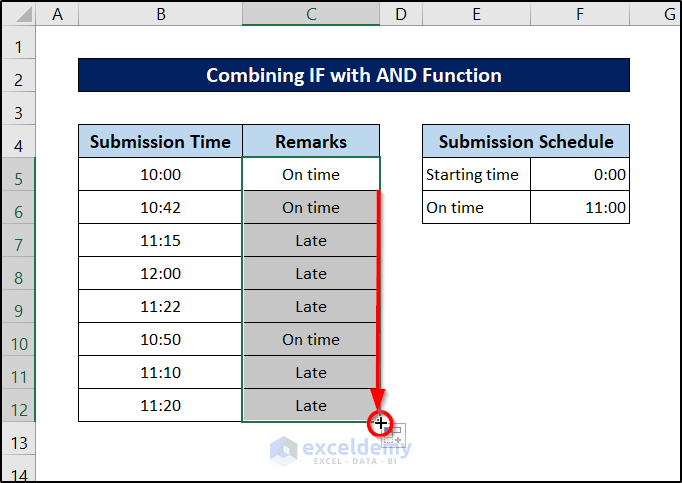
This is the output.
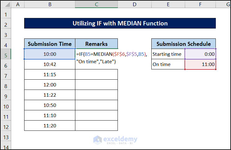
Example 5 – Utilizing the IF with the MEDIAN Function
Steps:
- Select a cell to see the result. Here, C5.
- Enter the following formula.
=IF(B5=MEDIAN($F$6,$F$5,B5),"On time","Late")
Formula Breakdown
IF(B5=MEDIAN($F$6,$F$5,B5),”On time”,”Late”)
MEDIAN($F$6,$F$5,B5) determines the median between the cell values of F6, F5, and B5.
IF(B5=MEDIAN($F$6,$F$5,B5),”On time”,”Late”) checks whether the value of B5 is equal to the median. If it is, the function returns “On time”. Otherwise, it returns “Late”.
- Press Enter.
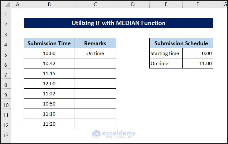
- Drag down the Fill Handle to see the result in the rest of the cells.
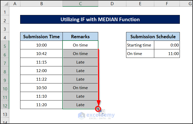
This is the output.
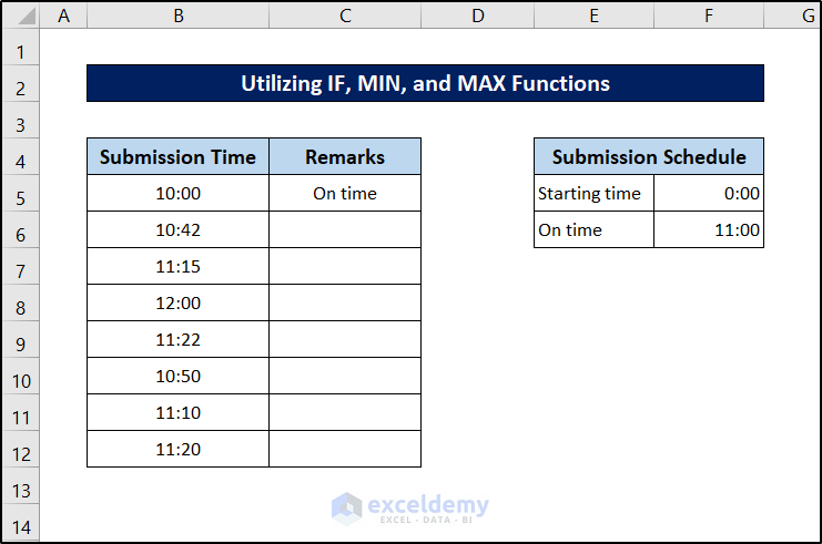
Example 6 – Utilizing the IF, MIN and MAX Functions
Steps:
- Select a cell to see the result. Here, C5.
- Enter the following formula.
=IF(AND(B5>=MIN($F$5:$F$6),B5<=MAX($F$5:$F$6)),"On time","Late")

Formula Breakdown
IF(AND(B5>=MIN($F$5:$F$6),B5<=MAX($F$5:$F$6)),”On time”,”Late”)
MIN($F$5:$F$6 determines the minimum value in F5:F6.
MAX($F$5:$F$6) returns the maximum value in F5:F6.
AND(B5>=MIN($F$5:$F$6),B5<=MAX($F$5:$F$6)) checks whether the value of B5 is greater than or equal to the minimum value of F5:F6 and less than or equal to the maximum value of F5:F6. The function returns TRUE if both conditions are met. Otherwise, FALSE.
IF(AND(B5>=MIN($F$5:$F$6),B5<=MAX($F$5:$F$6)),”On time”,”Late”) takes the previous function as the condition that returns a boolean result. The function returns “On time” or “Late”, depending on whether the previous function returned TRUE or FALSE.
- Press Enter.
- Drag down the Fill Handle to see the result in the rest of the cells.

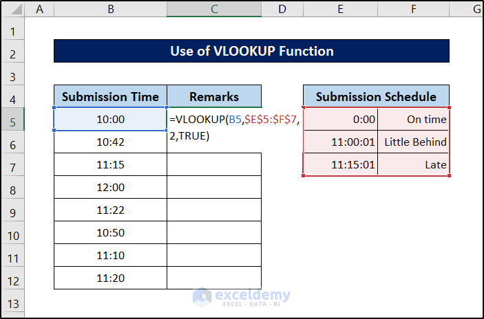
Example 7 – Using the VLOOKUP Function

Steps:
- Select a cell to see the result. Here, C5.
- Enter the following formula.
=VLOOKUP(B5,$E$5:$F$7,2,TRUE)
- Press Enter.
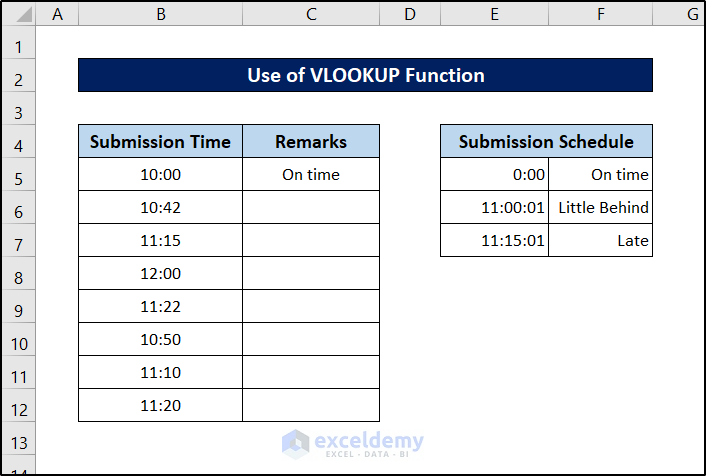
- Drag down the Fill Handle to see the result in the rest of the cells.

This is the output.
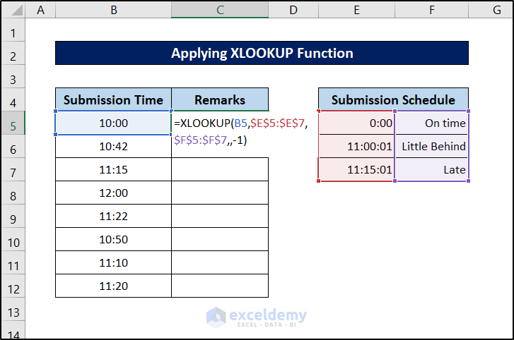
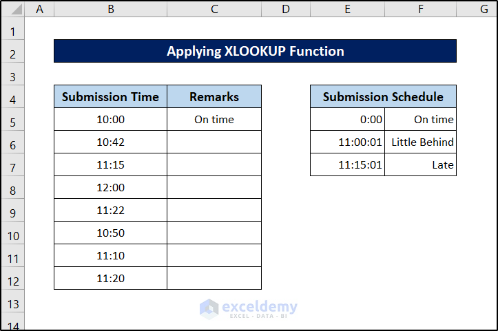
Example 8 – Applying the XLOOKUP Function
Steps:
- Select a cell to see the result. Here, C5.
- Enter the following formula.
=XLOOKUP(B5,$E$5:$E$7,$F$5:$F$7,,-1)
- Press Enter.
- Drag down the Fill Handle to see the result in the rest of the cells.
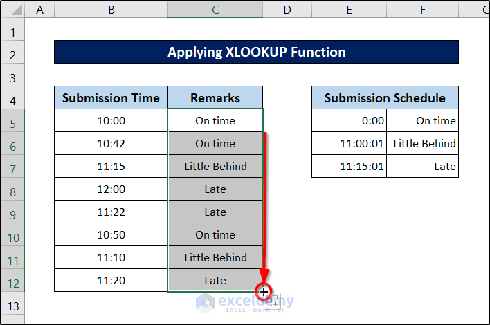
This is the output.
Download Practice Workbook
Download the workbook.
<< Go Back to If Time Between Range | Formula List | Learn Excel
Get FREE Advanced Excel Exercises with Solutions!
