Excel Change Color If Time Is in Range: 3 Suitable Ways

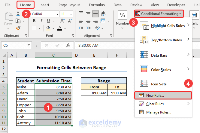
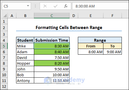
Method 1 – Formatting Cells Between Time Range to Change Color

• Select the range of cells > go to the Home tab > click Conditional Formatting > select New Rule.

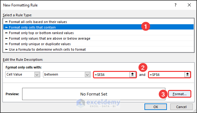
• The New Formatting Rule dialog box will appear.
• Choose Format only cells that contain from the Select a Rule Type field.
• In our dataset, cell E5 contains the starting range and cell F5 contains the ending range.
• In the Format only cells with section, enter your starting and ending range.
• Click Format feature to choose a color to format cells.

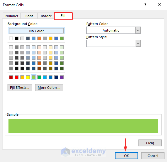
• In the appeared Format Cells dialog box, go to the Fill section > choose a color > click OK.

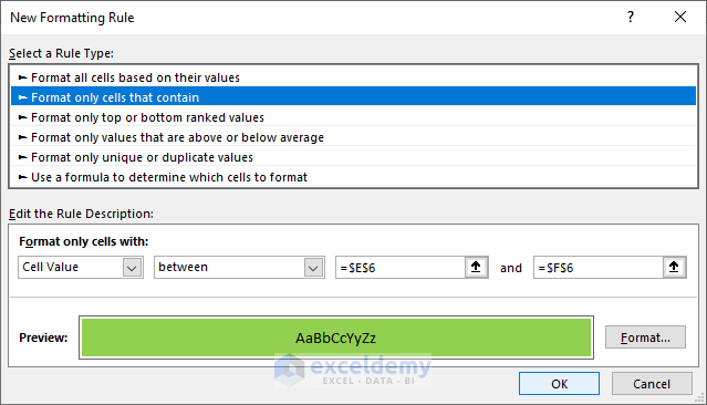
• Close the New Formatting Rule dialog box by clicking OK.

• The selected cells whose values are in the specified range will change their color.

Method 2 – Use Formula in Conditional Formatting to Change Color Based on Time

• Select the range of cells and again launch the New Formatting Rule dialog box.
• Choose Use a formula to determine which cells to format from the Select a Rule Type field.
• Apply the formula in the “Format values where this formula is true” field and choose a color. We used the AND function in the formula as we had to match our values between two values.

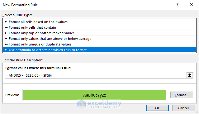
• Excel will change the cell color.

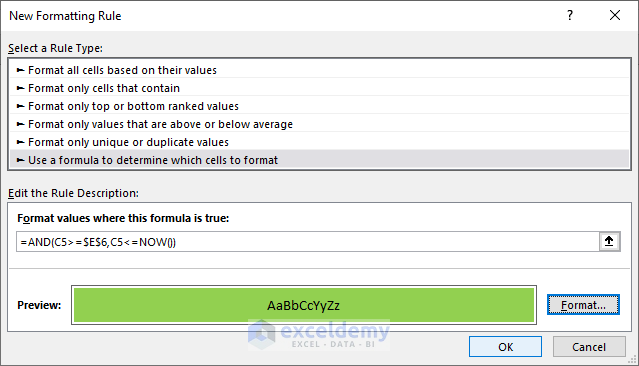
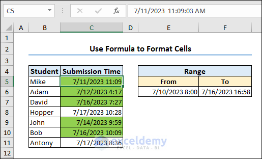
Method 3 – Use Formula in Conditional Formatting to Change Color Based on Date and Time

This formula finds whether cell C5 has a value between the value of cell E6 and the value returned by the NOW function.

Get the cell color changed.

How to Change Color Based on Date in Excel

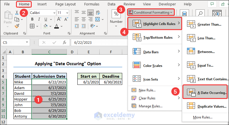
Method 1 – Apply the “Date Occurring” Option of Conditional Formatting for Dates

• Select the range containing dates > go to the Home tab > click Conditional Formatting > select Highlight Cells Rules > click A Date Occurring option.

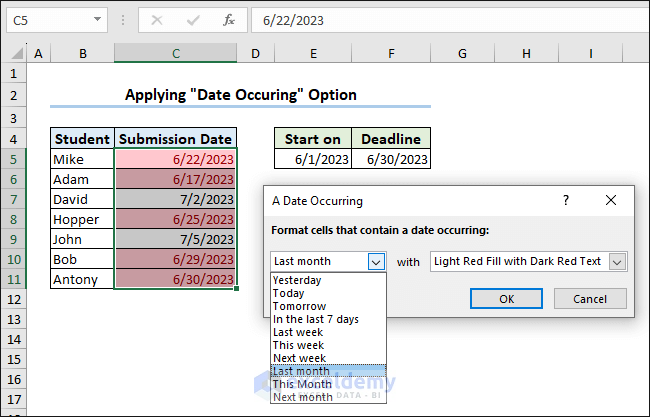
• NA Date Occurring dialog box will appear.
• Find several options for dates from which you can choose (i.e. Last Month). Based on your choice, this command will change the cell color. As we have chosen Last Month, Excel will change the dates of the last month.

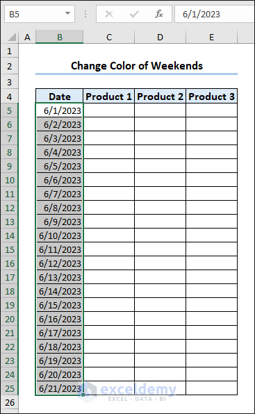
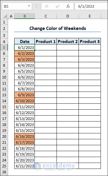
Method 2 – Change the Color of Cells for Weekends

• Select the range of dates.

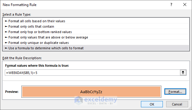
• The New Formatting Rule dialog box.
• Apply the following formula:

• Excel will change the cell color on the weekends.

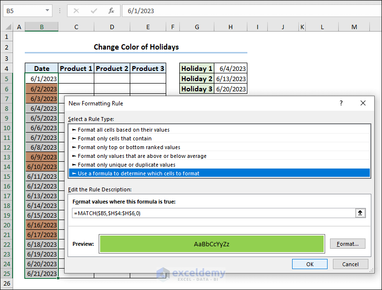
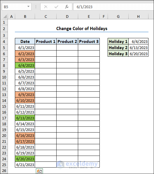
Method 3 – Highlight Holidays in Excel

We have specified some weekends in the dataset: 6/4/2023, 6/13/2023, 6/20/2023. On the previously weekend highlighted sheet, now apply the MATCH function to highlight the holidays:

This formula will match the dates with the holidays specified in the range $H$4:$H$6.

The dates which match with the specified holiday will now change their color.

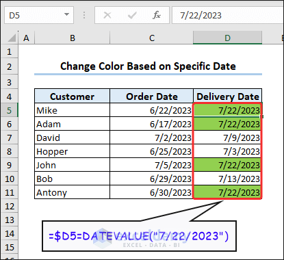
Method 4 – Change Cell Color Based on a Specific Date

The syntax of the DATEVALUE function is:

The argument date_text is: date in text format.

Apply the following formula in conditional formatting:

This formula finds the date value of “7/22/2023” in column D and highlights the cell values that match with “7/22/2023”.

Method 5 – Change the Cell Color of Dates Based on Today

To highlight the cell containing the date of today, apply the TODAY function in the conditional formula. The TODAY function returns the current date formatted as the date.

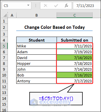
Method 6 – Highlight Dates Based on Multiple Criteria

If you want to highlight the whole rows where both the “Repeat” customers and order date are greater than today (7/19/2023):

• Select the full range of datasets and apply the following formula in the conditional formatting:

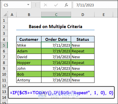
Method 7 – Highlight Upcoming and Previous Dates

If you want to highlight 10 upcoming days from today’s date, apply the following formula in the conditional formatting.

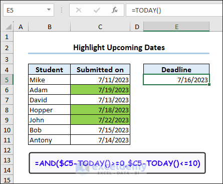
Highlight the 10 previous days from today’s date, and apply the following formula in the conditional formatting.

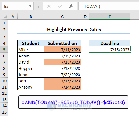
Key Takeaways from the Article

• Conditional formatting in Excel allows you to change the color of cells based on specific time ranges.
• Conditional formatting is a dynamic feature in Excel. So, if the time values change, the cell colors will automatically update to reflect the new conditions.
• AND function is particularly useful when setting up conditional formatting for time ranges.
• Conditional formatting is not limited to time ranges. You can also apply it for a date range.

Download Practice Workbook

You can download the practice workbook from the link below.

Frequently Asked Questions

1. Can I apply conditional formatting to highlight time ranges in Excel for both single cells and cell ranges?

Ans: Yes, you can apply conditional formatting to highlight time ranges in Excel for both single cells and cell ranges.

2. Is it possible to create dynamic time ranges for conditional formatting in Excel, such as based on a changing reference cell?

Ans: Yes, by using formulas and cell references within the conditional formatting rules, you can dynamically adjust the time ranges based on the value of a reference cell.

3. How can I remove or clear conditional formatting rules that have been applied to time-based cells in Excel?

Ans: To remove conditional formatting rules from time-based cells in Excel, select the cells, go to the Home tab > click Conditional Formatting > and choose Clear Rules from the drop-down menu.

<< Go Back to If Time Between Range | Formula List | Learn Excel