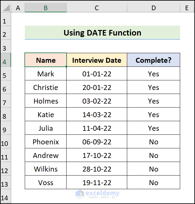
Consider the Interview Schedule dataset in the B4:C13 cells below, with Names of the employees and their scheduled Interview Dates. To determine whether the candidates have been interviewed, use one of the following date-based functions.

Method 1 – Using DATEVALUE Function to Return Value If Cell Contains Date
Steps:
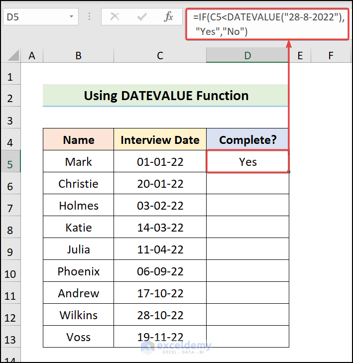
- Go to the D5 cell and enter the following formula:
=IF(C5<DATEVALUE("28-8-2022"),"Yes","No")
Here, the C5 cell refers to the Interview Date 01-01-22 while the hard-coded checking date is 28-08-22.
Formula Breakdown:
- DATEVALUE(“28-8-2022”) → converts a date in the form of text to a number that represents the date in Microsoft Excel date-time code. Here, “28-8-2022” is the date_text argument which is today’s date and Excel returns the date in numerical format.
- Output → 44801 (number of days after Jan 1, 1900)
- IF(C5<DATEVALUE(“28-8-2022″),”Yes”,”No”) → checks whether a condition is met and returns one value if TRUE and another value if FALSE. Here, C5<DATEVALUE(“28-8-2022”) is compares the date in the C5 cell with the checking date. If C5 is lower the function returns “Yes” (value_if_true argument), otherwise it returns “No” (value_if_false argument).
- Output for D5 → Yes
- Use the Fill Handle Tool to copy the formula into the cells below.
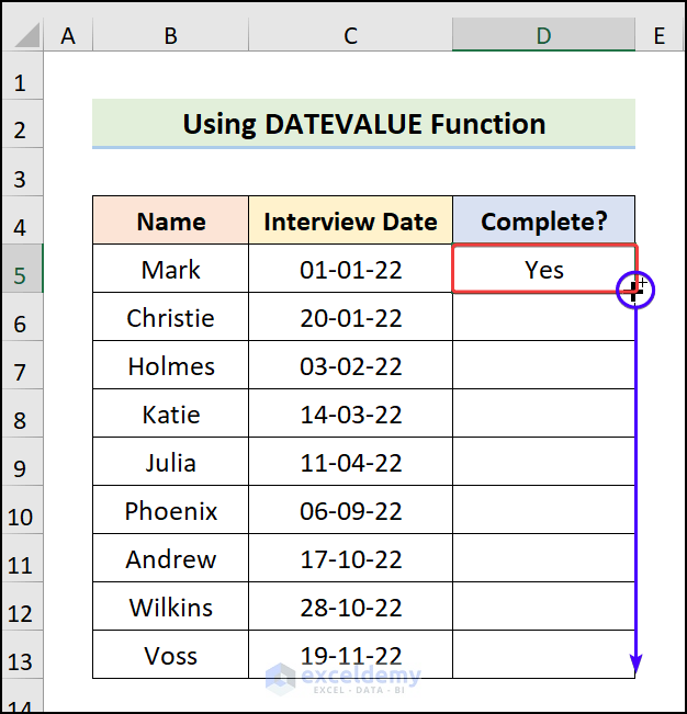
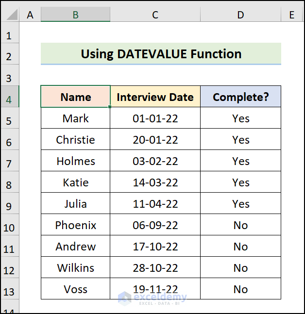
Finally, your result should look like the image shown below.
Method 2 – Returning Value with DATE Function If Cell Contains Date
Steps:
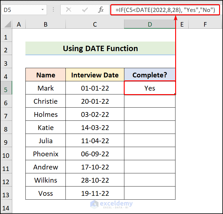
- Go to the D5 cell and type in the expression given below:
=IF(C5<DATE(2022,8,28), "Yes","No")
Formula Breakdown:
- DATE(2022,8,28) → returns the number that represents the date in Microsoft Excel date-time code. Here, 2022 is the year argument, next 8 is the month argument, and 28 is the day argument.
- Output → 28-08-22
- IF(C5<DATE(2022,8,28), “Yes”,”No”) → checks whether a condition is met and returns one value if TRUE and another value if FALSE. Here, C5<DATE(2022,8,28) is the logical_test argument that compares the date in the C5 cell with the given date. If this value is less than the given date then the function returns “Yes” (value_if_true argument) otherwise it returns “No” (value_if_false argument).
- Output → Yes
- Move the Fill Handle from D5 down to copy the formula across the column.
Method 3 – Utilizing TODAY Function to Return Value If Cell Contains Date
Steps:
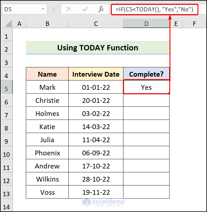
- Go to the D5 cell and enter the following formula.
=IF(C5<TODAY(), "Yes","No")
Formula Breakdown:
- TODAY() → returns the current date formatted as a date.
- IF(C5<TODAY(), “Yes”,”No”) → checks whether a condition is met and returns one value if TRUE and another value if FALSE. Here, C5<TODAY() is the logical_test argument that compares the date in the C5 cell with today’s date. If this value is less than the today’s date then the function returns “Yes” (value_if_true argument) otherwise it returns “No” (value_if_false argument).
- Output → Yes
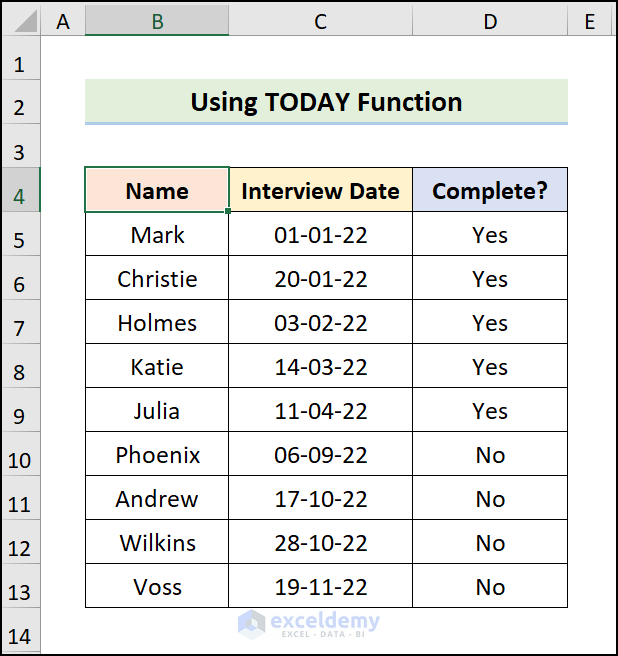
- Once you drag the Fill Handle down, your output should look like the screenshot given below.
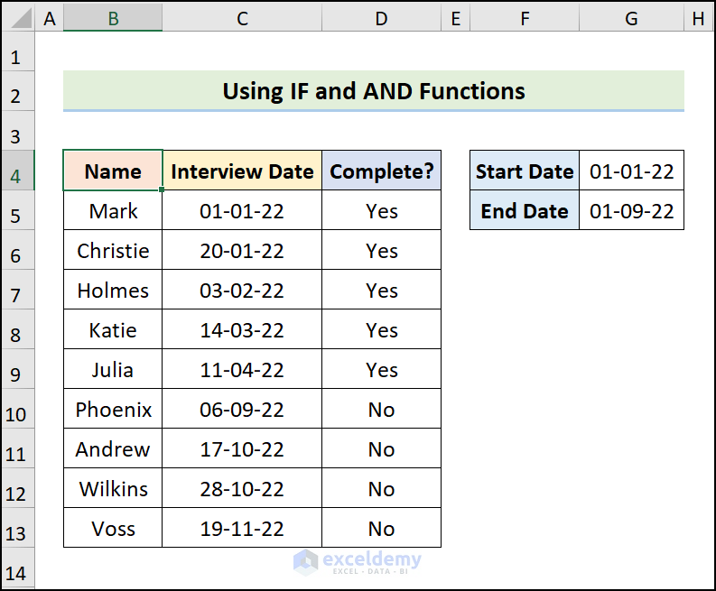
Method 4 – Combining IF and AND Functions to Return Value Between Two Dates
Steps:
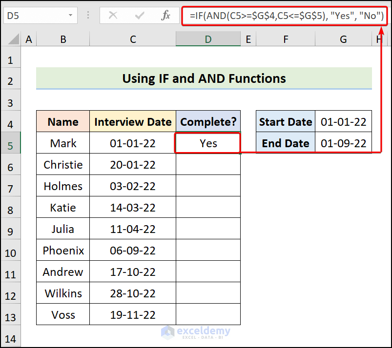
- Type in the formula provided below into cell D5:
=IF(AND(C5>=$G$4,C5<=$G$5), "Yes", "No")
Here, the G4 and G5 cells point to the Start Date and the End Date respectively. Make sure to use Absolute Cell Reference by pressing the F4 key on your keyboard or using $ symbols.
Formula Breakdown:
- AND(C5>=$G$4,C5<=$G$5) → returns TRUE only if all the arguments are TRUE. Since both C5>=$G$4 and C5<=$G$5 are TRUE so the AND function results in TRUE.
- Output → TRUE
- IF(AND(C5>=$G$4,C5<=$G$5), “Yes”, “No”) → Since AND(C5>=$G$4,C5<=$G$5) is the logical_test and is TRUE, then the function returns “Yes” (value_if_true argument).
- Output → Yes
- Drag the FIll Handle down from D5 to other cells in the column and the results should appear like the image below.
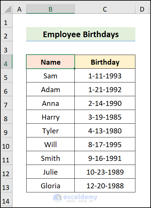
Method 5 – Applying COUNTIFS Function to Return Value If Cell Contains Specific Date
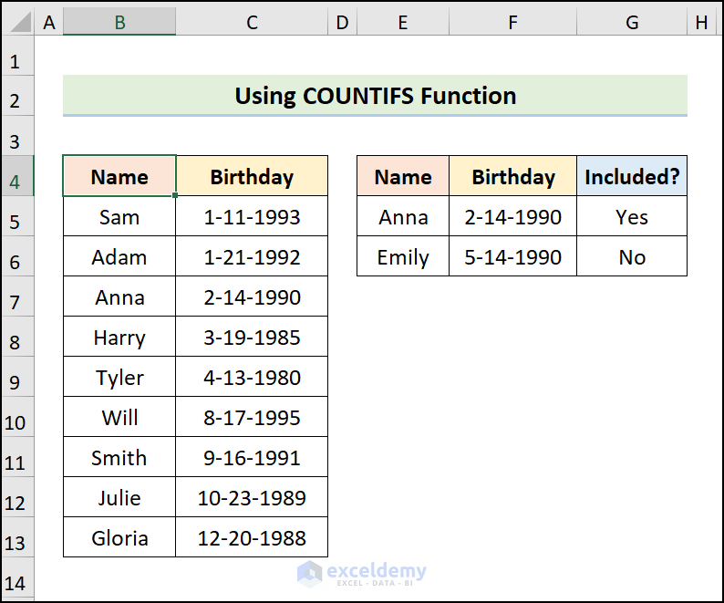
Let’s use the Employee Birthdays dataset shown in the B4:C13 cells below to check whether a test value is in the table.
Steps:
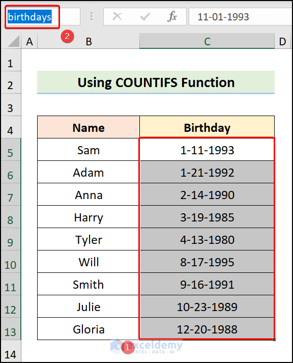
- Select the C4:C13 cells.
- Double-click the Name Box.
- Enter a suitable name for this range of cells, such as birthdays.
- Select the G5 cell and enter the formula below:
=IF(COUNTIFS(birthdays,F5)>0, "Yes", "No")
The F5 cell will be the cell with the testing date.
Formula Breakdown:
- COUNTIFS(birthdays,F5) → counts how many cells in the birthdays range have the same value as F5.
- IF(COUNTIFS(birthdays,F5)>0, “Yes”, “No”) → COUNTIFS(birthdays,F5)>0 will be true if the COUNTIFS function finds an F5 among the testing range. If it does, the whole function will output “Yes.” Otherwise, the output will be “No.”
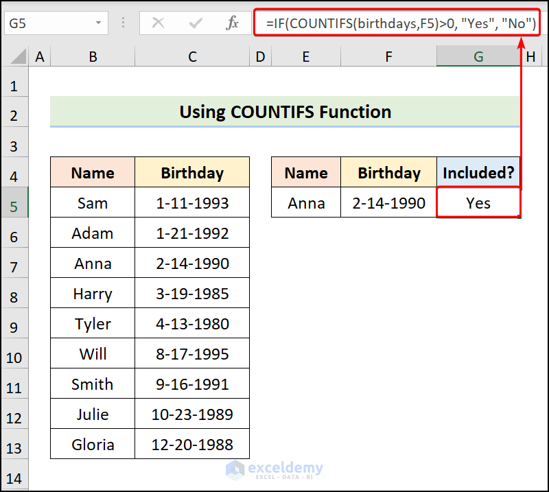
- Copy the same formula to the cell below. Based on the example below, the birthday of Emily is not present in the original list so the function returns a No.
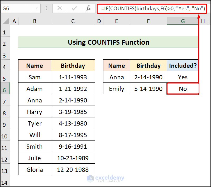
Consequently, the output should look like the picture shown below.
If Cell Contains Date Then Apply Conditional Formatting
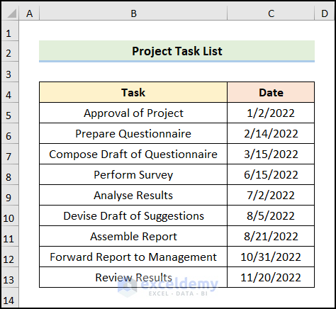
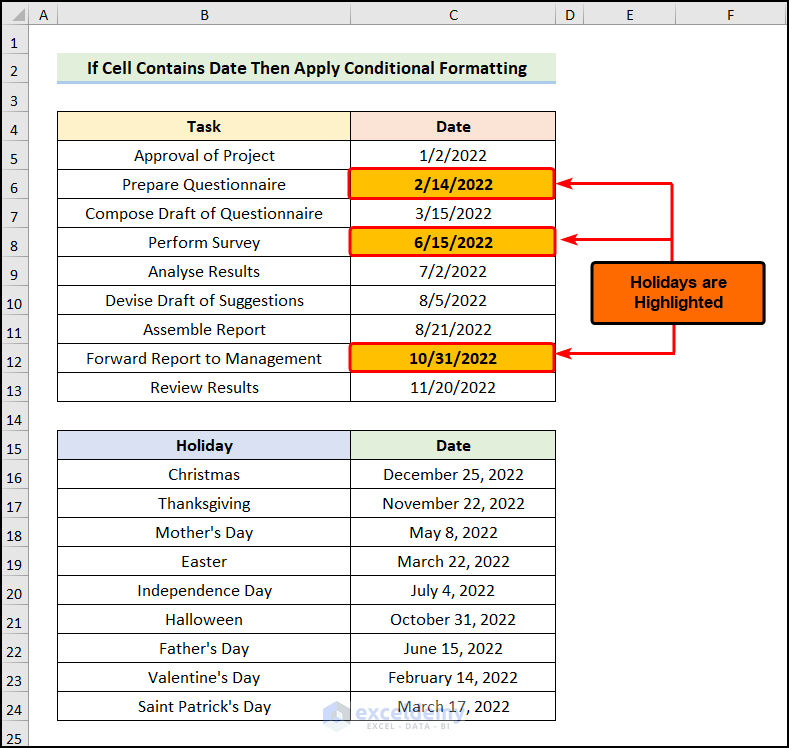
You can also use Conditional Formatting based on date cells. Consider the Project Task List dataset shown in the B4:C13 below, with the task to highlight cells in the Date column which coincide with given Holiday Dates.
Steps:
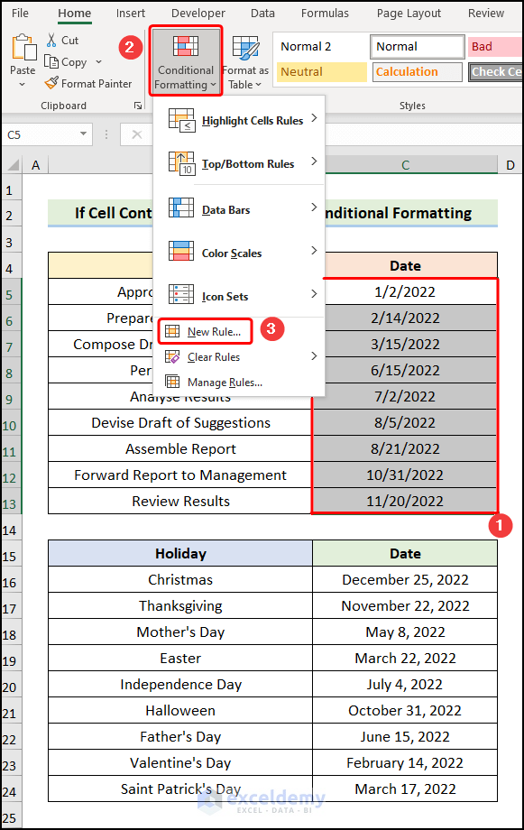
- Select the C5:C13 cells.
- Go to the Conditional Formatting drop-down. c
- Choose the New Rule option.
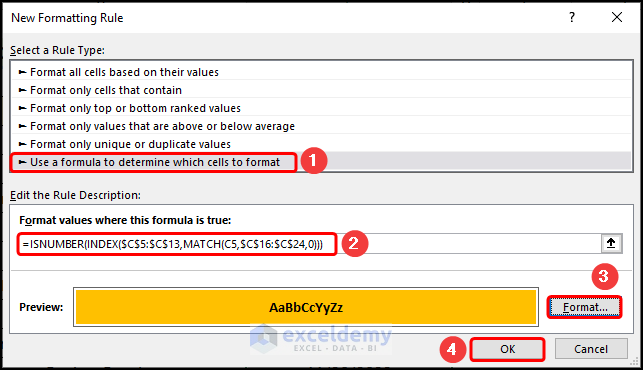
- Choose the Use a formula to determine which cells to format option in the wizard.
- In the Rule Description box, enter the following formula:
=ISNUMBER(INDEX($C$5:$C$13,MATCH(C5,$C$16:$C$24,0)))
Here, the C5 cell points to the Project Approval Date while the $C$5:$C$13 and $C$16:$C$24 ranges represent the Dates for the Task and Holidays.
Formula Breakdown:
- MATCH(C5,$C$16:$C$24,0)) →The MATCH function returns the relative position of an item in an array matching the given value. Here, C5 is the lookup_value argument that refers to the Project Approval Date. Following, $C$16:$C$24 represents the lookup_array argument from where the value is matched. Lastly, 0 is the optional match_type argument which indicates the Exact match criteria.
- Output → #N/A
- INDEX($C$5:$C$13,MATCH(C5,$C$16:$C$24,0)) → becomes
- INDEX($C$5:$C$13,#N/A) →The INDEX function returns a value at the intersection of a row and column in a given range. In this expression, the $C$5:$C$13 is the array argument which are the Task Dates. Next, #N/A is the row_num argument that indicates that the Date is not present.
- Output → #N/A
- ISNUMBER(INDEX($C$5:$C$13,MATCH(C5,$C$16:$C$24,0))) → becomes
- ISNUMBER(#N/A) →The ISNUMBER function checks whether a value is a number and returns TRUE or FALSE. Here, #N/A is the value argument, and since it is not a number so the function returns FALSE.
- Output → FALSE
Note: Please make sure to use Absolute Cell References by pressing the F4 key on your keyboard.
Now, you can see the entire procedure in the GIF below.
This should highlight the Holidays in bright orange color.
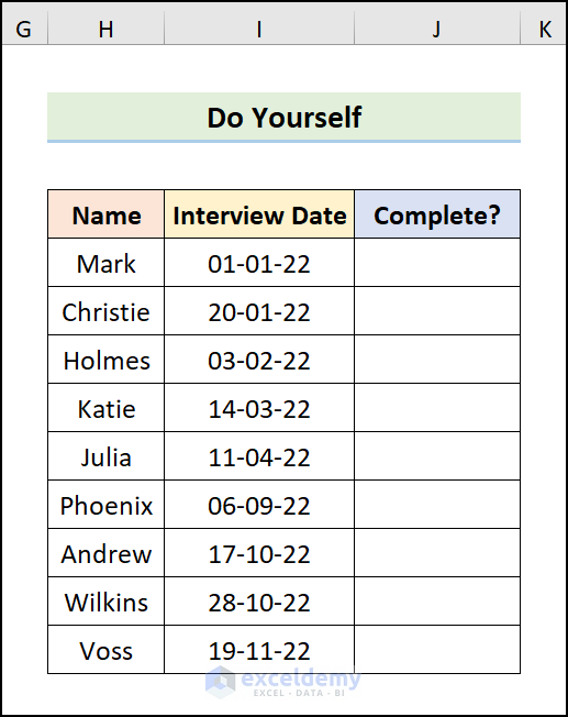
Practice Section
The sample below contains a Practice section on the right side of each sheet so you can practice.
Download Practice Workbook
You can download the practice workbook from the link.
<< Go Back to If Date | Formula List | Learn Excel
Get FREE Advanced Excel Exercises with Solutions!
