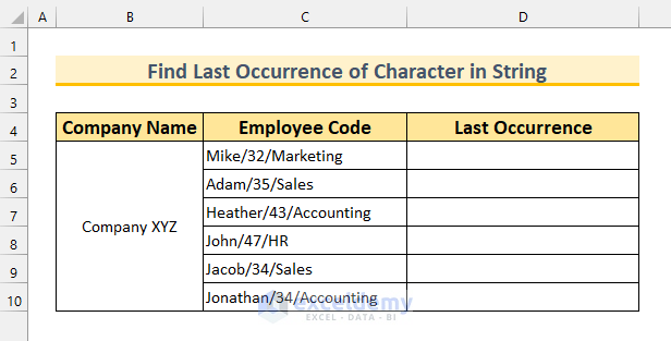
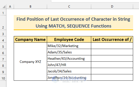
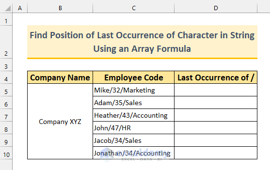
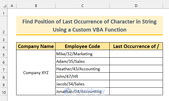
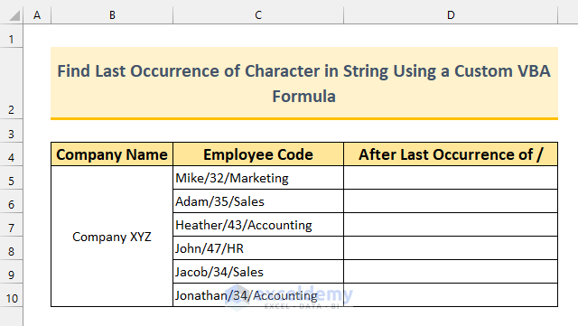
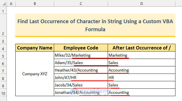
Our sample dataset has three columns: Company Name, Employee Code, and Last Occurrence. Employee Code contains the name, age, and department of an employee. For the first 5 methods, we’ll find the position of the forward-slash “/” in for all the values in the Employee Code. After that, we’re going to output strings after the last slash in the last 3 methods.
Excel Find Last Occurrence of Character in String: 8 Methods
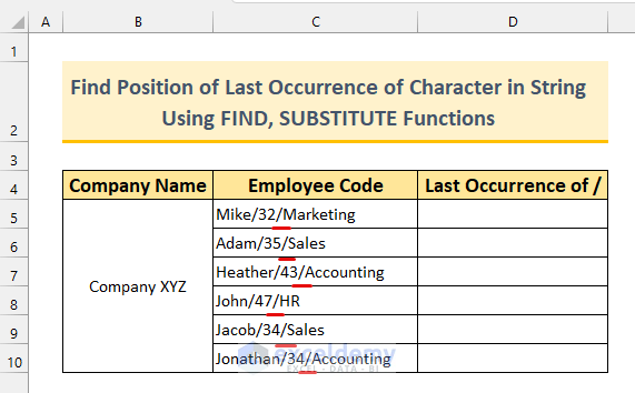
Method 1 – Using FIND & SUBSTITUTE Functions in Excel to Find Position of Last Occurrence of Character in String
Let’s extract the position of the final slash in the codes from the dataset.
Steps:
- Copy the following formula in cell D5.
=FIND(CHAR(134),SUBSTITUTE(C5,"/",CHAR(134),(LEN(C5)-LEN(SUBSTITUTE(C5,"/","")))/LEN("/")))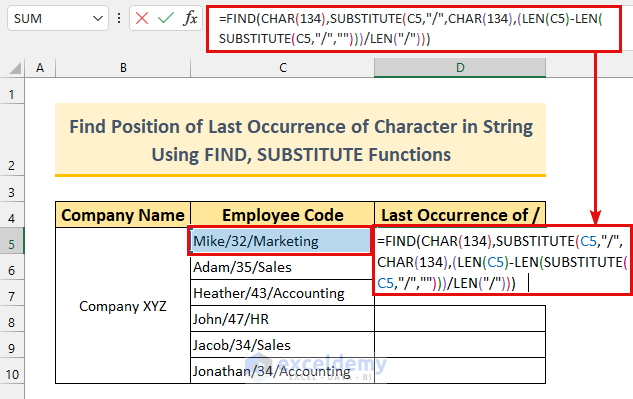
Formula Breakdown
Our main function is FIND. We’re going to find the CHAR(134) value in our string.
- CHAR(134)
- Output: †.
- We need to set a character that is not present in our strings. We’ve chosen it because it is rare in strings. If somehow you have this in your strings, change it to anything that is not in your strings (for example “@”, “~”, etc.).
- SUBSTITUTE(C5,”/”,CHAR(134),(LEN(C5)-LEN(SUBSTITUTE(C5,”/”,””)))/LEN(“/”)) -> becomes,
- SUBSTITUTE(C5,”/”,”†”,(17-LEN(“Mike32Marketing”))/1) -> becomes,
- SUBSTITUTE(“Mike/32/Marketing”,”/”,”†”,(17-15)/1)
- Output: “Mike/32†Marketing”.
- Now our full formula becomes,
- =FIND(“†”,”Mike/32†Marketing”)
- Output: 8.
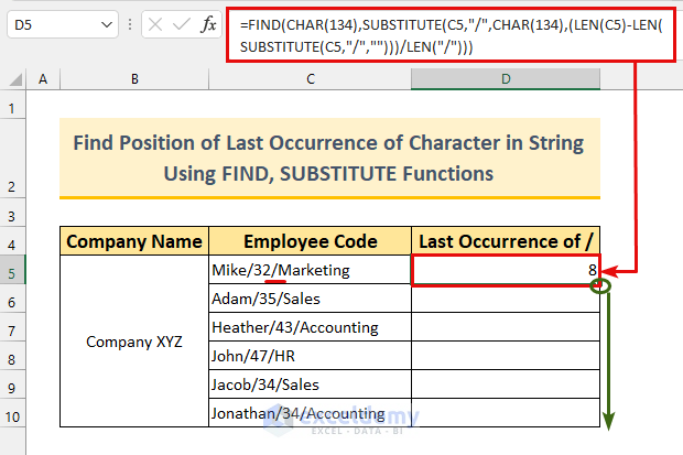
- Press Enter.
We’ll see the value 8. If we count manually from the left side, we will get 8 as the position for the slash in cell C5.
- Use the Fill Handle to copy the formula down.
Thus, we’ve got the position of the last occurrence of a character in our string.

Method 2 – Applying MATCH & SEQUENCE Functions in Excel to Find Position of Last Occurrence of Character in String
The SEQUENCE function is only available on Excel 365 or Excel 2021. We’ll use the same dataset.
Steps:
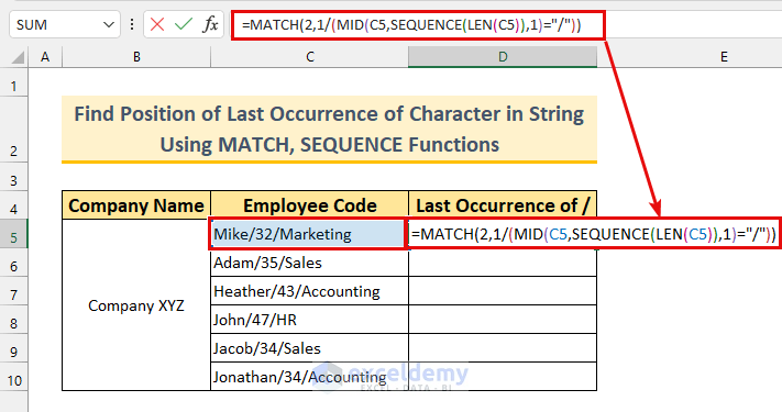
- Insert the following formula in cell D5:
=MATCH(2,1/(MID(C5,SEQUENCE(LEN(C5)),1)="/"))- SEQUENCE(LEN(C5))
- Output: {1;2;3;4;5;6;7;8;9;10;11;12;13;14;15;16;17}.
- The LEN function measures the length of cell C5. The SEQUENCE function returns a list of numbers sequentially in an array.
- MATCH(2,1/(MID(C5,{1;2;3;4;5;6;7;8;9;10;11;12;13;14;15;16;17},1)=”/”))
- Output: 8.
- The Match function is finding the last 1 value in our formula. It is in the 8th position.
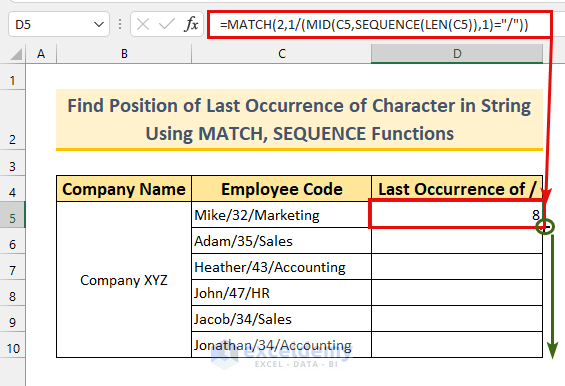
- Press Enter.
Using the formula, we’ve found the position of forward-slash as 8 in our string.
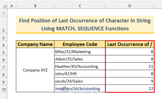
- Use the Fill Handle to AutoFill the formula.
This finds the last position of a character in the strings.
Read More: How to Find Character in String Excel
Method 3 – Utilizing an Array Formula in Excel to Find Position of Last Occurrence of Character in String
We’re going to use the ROW function, the INDEX function, the MATCH, the MID, and the LEN functions to create an array formula to find the position of the last occurrence of a character in a string.
Steps:
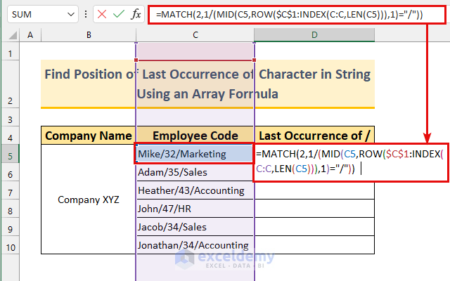
- Input the formula below into cell D5:
=MATCH(2,1/(MID(C5,ROW($C$1:INDEX(C:C,LEN(C5))),1)="/"))Formula Breakdown
The formula is similar to method 2. We’re using the ROW and the INDEX function to replicate the output as the SEQUENCE function.
- ROW($C$1:INDEX(C:C,LEN(C5)))
- Output: {1;2;3;4;5;6;7;8;9;10;11;12;13;14;15;16;17}.
- We can see the output is the same. The INDEX function returns the value of a range. The LEN function is counting the length of the string from cell C5. Finally, the ROW function is returning the cell values from 1 to the cell length of C5. The rest of the formula is the same as method 2.
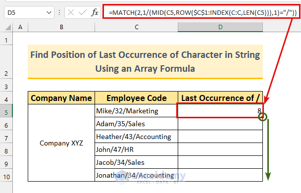
- Press Enter.
We’ve got 8 as the value as expected. Our formula worked flawlessly.
Note: We’re using the Excel 365 version. If you’re using an older version, then you will need to press Ctrl + Shift + Enter.
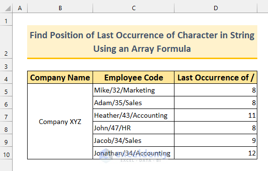
- Double-click or drag down the Fill Handle.
- This is what the final result should look like.
Read More: How to Find Character in String from Right in Excel
Method 4 – User Defined Function to Find Position of Last Occurrence of Character in String
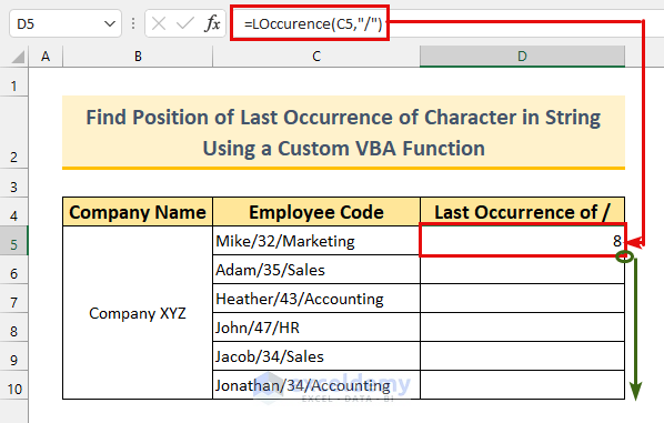
In this method, we will use a custom VBA formula to find the last position of a character in a string.
Steps:
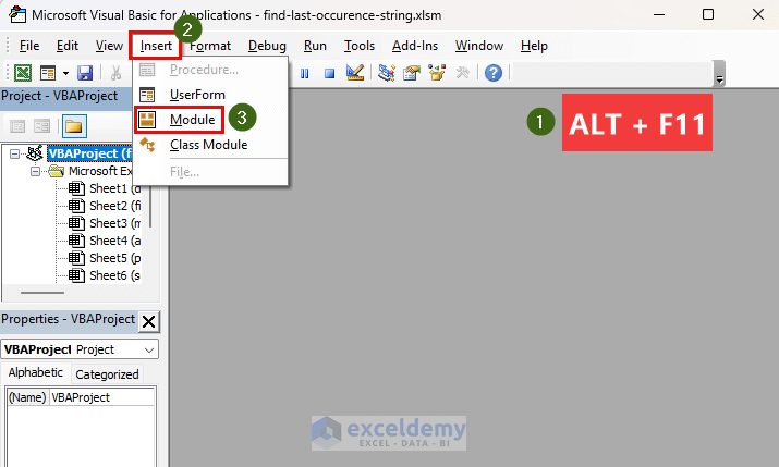
- Press Alt + F11 to bring up the VBA window. You can choose Visual Basic from the Developer tab, as well.
- From Insert, select Module.
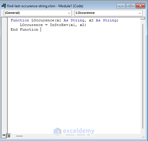
- Copy and paste the following code into the module:
Function LOccurence(x1 As String, x2 As String)
LOccurence = InStrRev(x1, x2)
End Function
We’ve created a custom function called “LOccurence”. The InStrRev is a VBA function that returns the end position of a character. We’ll input our cell value as x1 and the specific character (in our case, it is a forward-slash) as x2 in this custom function.
- Close the VBA window and go to the “Position VBA” sheet.
- Type the following formula in cell D5:
=LOccurence(C5,"/")In this custom function, we’re telling it to find the position of the last occurrence of forward-slash in the string from cell C5.
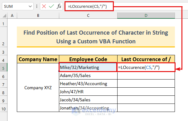
- Press Enter.
We’ve got 8 as expected as the last occurred position of the forward-slash.
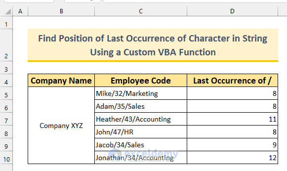
- Drag the formula down using the Fill Handle.
- Here’s the final result.
Read More: How to Find from Right in Excel
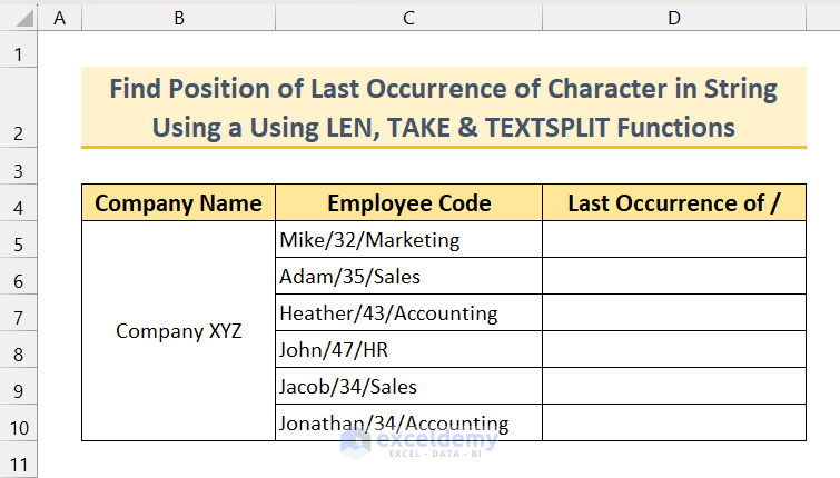
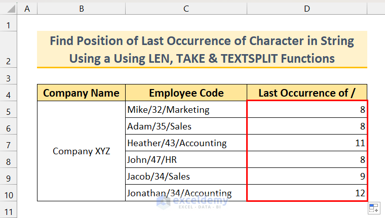
Method 5 – Using LEN, TAKE & TEXTSPLIT Functions to Find Position of Last Occurrence of Character in String in Excel
The TAKE and TEXTSPLIT functions are only available in Excel for Microsoft 365.
Steps:
- Insert the following formula in cell D5:
=LEN(C5)-LEN(TAKE(TEXTSPLIT(C5,"/"),1,-1))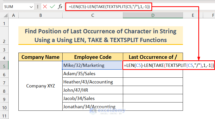
Formula Breakdown
- TEXTSPLIT(C5,”/”)
Splits cell C5 around the delimiter “/” and returns the array (Mike 32 Marketing).
- TAKE(TEXTSPLIT(C5,”/”),1,-1))
Returns only the last element (i.e. Marketing) from the array (Mike 32 Marketing)
- LEN(TAKE(TEXTSPLIT(C5,”/”),1,-1))
Returns the length of the string Marketing. Output: 9
- LEN(C5)
Returns the length of the string in cell C5. Output: 17
- LEN(C5)-LEN(TAKE(TEXTSPLIT(C5,”/”),1,-1))
This difference refers to the position of the last occurrence of the character “/”.
- Press the Enter key and drag down the Fill Handle icon.
![]()
- Here is the final output of the last occurring positions of the “/” character.
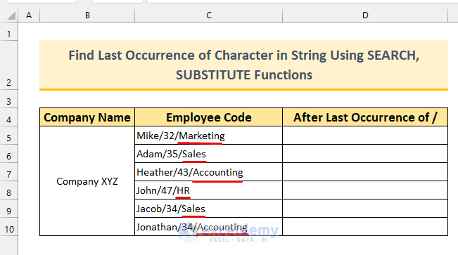
Method 6 – Using Combined Functions in Excel to Find Last Occurrence of Character in String
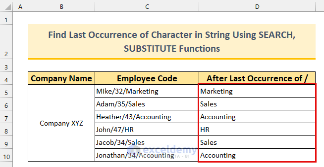
We’re going to use the SEARCH function, the RIGHT function, the SUBSTITUTE, the LEN, the CHAR functions to show the string after the last occurrence of a character, so we’ll output the department of the employees from the Employee Code column.
Steps:
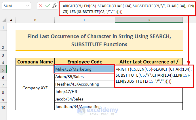
- Insert the following formula in cell D5:
=RIGHT(C5,LEN(C5)-SEARCH(CHAR(134),SUBSTITUTE(C5,"/",CHAR(134),LEN(C5)-LEN(SUBSTITUTE(C5,"/","")))))Formula Breakdown
- SUBSTITUTE(C5,”/”,CHAR(134),LEN(C5)-LEN(SUBSTITUTE(C5,”/”,””))) -> becomes,
- SUBSTITUTE(C5,”/”,CHAR(134),2)
- Output: “Mike/32†Marketing”.
- The SUBSTITUTE function replaces a value with another value. In our case, it is replacing each forward-slash with a † in the first portion and with blank in the latter portion. Then the LEN function measures the length of that. That is how we have got our value.
- SEARCH(“†”,”Mike/32†Marketing”)
- Output: 8.
- The SEARCH function is finding the special character in our previous output. Consequently, it found it in 8th
- Finally, our formula reduces to, RIGHT(C5,9)
- Output: “Marketing”.
- The RIGHT function returns the cell value up to a certain number of characters from the right side. We’ve found the position of the last forward-slash in 8th The length of cell C5 is 17, and 17–8 =9. Hence, we’ve got the 9 characters from the right side as the output.
- Press Enter.
We’ve gotten the strings after the last forward-slash.
- Use the Fill Handle to AutoFill the formulas into cell range D6:D10.
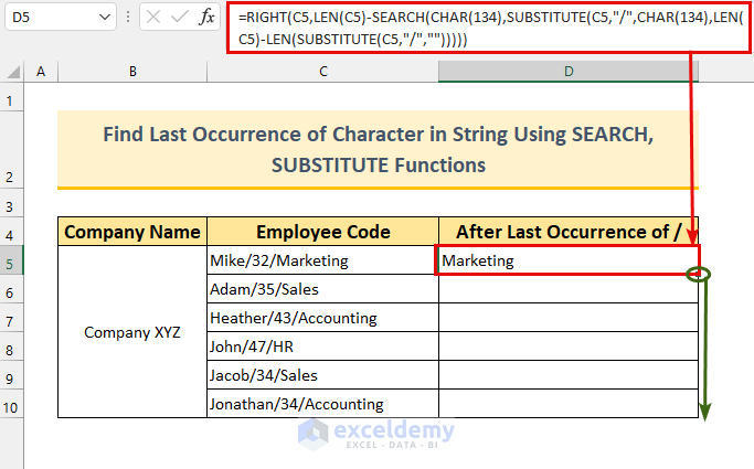
- This is the final result.
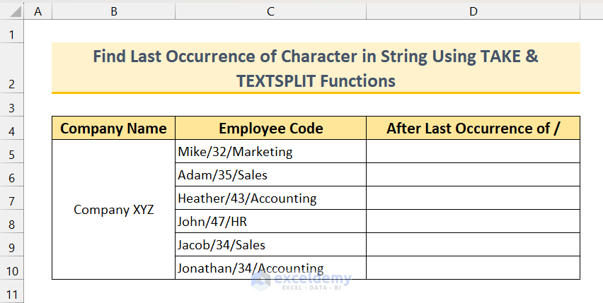
Method 7 – Applying TAKE & TEXTSPLIT Functions in Excel to Find Last Occurrence of Character in String
This method is similar to method 5.
Steps:
- In cell D5, copy and paste the following formula:
=TAKE(TEXTSPLIT(C5,"/"),1,-1)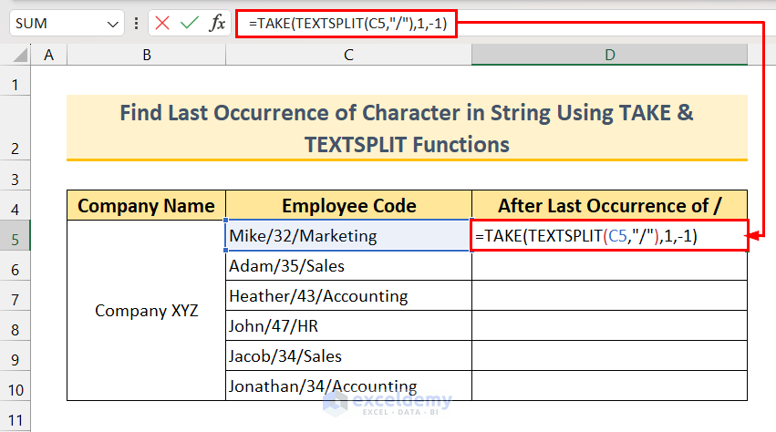
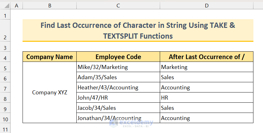
- Press the Enter key, then double-click on the Fill Handle icon.
![]()
- Here is the final output of the strings that appear after the last occurring positions of the “/” character.
Method 8 – Custom VBA Formula in Excel to Find Last Occurrence of Character in String
Let’s extract the department using a custom formula.
Steps:
- Press Alt + F11 to bring up the VBA window.
- From Insert, select Module.
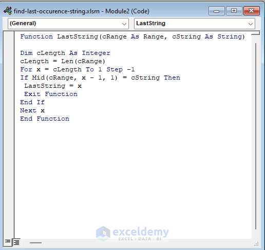
- Copy and paste the following code into the module window.
Function LastString(cRange As Range, cString As String)
Dim cLength As Integer
cLength = Len(cRange)
For x = cLength To 1 Step -1
If Mid(cRange, x - 1, 1) = cString Then
LastString = x
Exit Function
End If
Next x
End Function
We’re creating a custom function called “LastString”. This function will return the beginning position of the strings after the last occurrence of a character.
- Save the module.
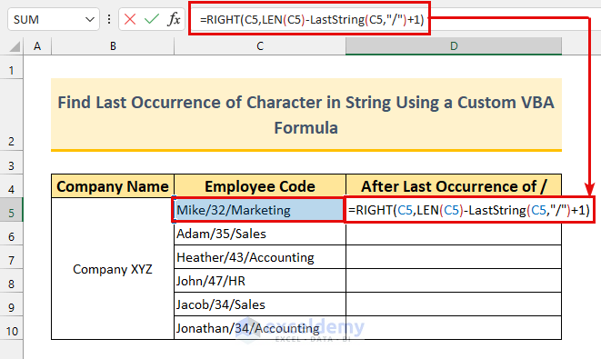
- Copy the formula from below to cell D5:
=RIGHT(C5,LEN(C5)-LastString(C5,"/")+1)Formula Breakdown
- LastString(C5,”/”)
- Output: 9.
- Here we’re getting the starting position of the string immediately after the last forward slash.
- LEN(C5)
- Output: 17.
- LEN(C5)-LastString(C5,”/”)+1
- Output: 9.
- We need to add 1 else we’ll get value with the “M”.
- Our formula will reduce to RIGHT(C5,9)
- Output: “Marketing“.
- Press Enter.
We’ll get the value “Marketing”.
- AutoFill the formula up to cell C10.
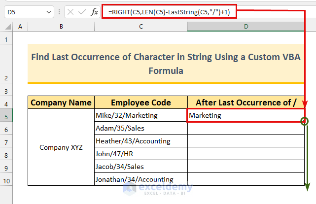
- Here’s the result.
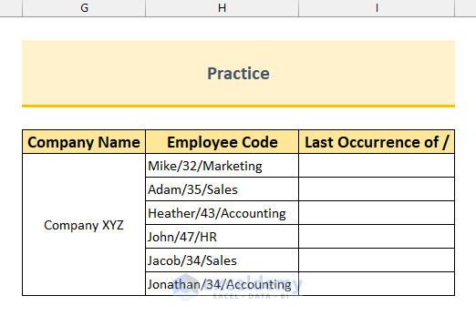
Practice Section
We’ve attached practice datasets beside each method in the Excel file.
Download Practice Workbook
Related Articles
- How to Find Text in Cell in Excel
- How to Check If Cell Contains Specific Text in Excel
- How to Find If Range of Cells Contains Specific Text in Excel
- How to Find * Character Not as Wildcard in Excel
<< Go Back to Find in String | String Manipulation | Learn Excel
Get FREE Advanced Excel Exercises with Solutions!

Two alternative formulae to find the last occurrence of a character in a string (cell C5):
1. In Excel 365
=FIND(MID(C5,LOOKUP(9^9,FIND(“/”,C5,SEQUENCE(LEN(C5)))),9^9),C5)
2. In earlier versions
=FIND(MID(C5,LOOKUP(9^9,FIND(“/”,C5,ROW(1:100))),9^9),C5)
Thanks for your formula.
Just a reminder, if anyone wants to copy and paste this formula, the quotes need to be straight (“”), not curly (“”). Otherwise, they will get the #N/A error.
1. Excel 365
=FIND(MID(C5,LOOKUP(9^9,FIND(“/”,C5,SEQUENCE(LEN(C5)))),9^9),C5)
2. Earlier Versions
=FIND(MID(C5,LOOKUP(9^9,FIND(“/”,C6,ROW(1:100))),9^9),C5)
Some additional options…
I feel like I found a much simpler way to achieve the result of method number 5 & 6 which only uses 2 functions:
=TAKE(TEXTSPLIT(C5,”/”),1,-1)
The TEXTSPLIT gives us an array, and the TAKE allows us to grab the last column.
Looks like these functions were added to Excel in 2022, so likely won’t work on older versions.
If the location of the last occurrence is needed instead (like in methods 1-4), we can add the use of LEN twice with a subtraction in between:
=LEN(C5)-LEN(TAKE(TEXTSPLIT(C5,”/”),1,-1))
Dear C2k,
Thanks for your feedback. Yes, you are right. Your mentioned formulas can achieve same results. But the TAKE and TEXTSPLIT functions in your formula are only available in Excel for Microsoft 365.
We have updated our article according to this method and mentioned the requirement of Microsoft 365. Thanks again.
Regards,
Seemanto Saha
ExcelDemy