How to Find from Right in Excel (6 Methods)

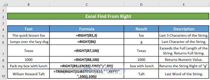
Let’s discuss how to use the Excel RIGHT function to find characters from the right in Excel.  Below is a summary of the formulae used in this tutorial.

Method 1 – Using the RIGHT Function

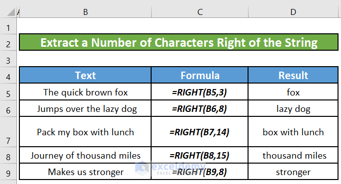
You can use the RIGHT function to extract a specific number of characters from the right of the string or text.

• Scenario:
  • Suppose we have a string in cell B5 that says “The quick brown fox”. We want to extract the last 3 characters from the right of this string (which corresponds to the word “fox”).

• Formula:
  • In an adjacent cell (let’s say D5), enter the following formula:

=RIGHT(B5,3)

• • B5 represents the cell containing the original string.
  • 3 specifies the number of characters to extract from the right.

• Result:
  • After entering the formula, cell D5 will display the extracted word fox.

• Repeat:
  • You can apply the same approach to other texts, adjusting the number of characters as needed.

Read More: How to Find Character in String from Right in Excel

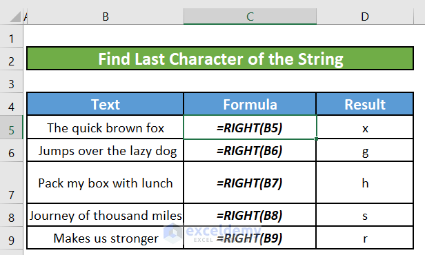
Method 2 -Extracting the Last Character of a String Using the RIGHT Function

• Scenario:
  • Suppose we have a string in cell B5 that says “The quick brown fox”. We want to extract the last character from this string (which corresponds to the letter “x”).

• Formula:
  • Instead of specifying the second argument (Num_chars), leave it empty. The formula for extracting only the last character will be as follows:

• • • B5 represents the cell containing the original string.

• Result:
  • After entering the formula, cell D5 will display the extracted character “x”.

Read More: Excel Find Last Occurrence of Character in String

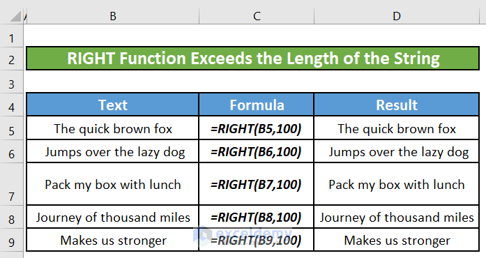
Method 3 – Handling Exceeding Length with the RIGHT Function

• Scenario:
  • If the second argument (Num_chars) exceeds the length of the string, the RIGHT function will return the entire text.

• Formula:
  • Let’s use the same formula but enter a large number (e.g., 100) for the second argument:

• Result:
  • Upon entering the formula, cell D5 will show the entire text from cell B5.

Read More: How to Find a Character in String in Excel

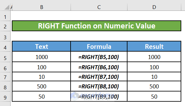
Method 4 – Applying the RIGHT Function to Numeric Values

• Scenario:
  • When applying the RIGHT function to a numeric value, it will return the same numeric value.

• Formula:
  • Use the same formula but apply it to a number:

• Result:
  • Cell D5 will display the same numeric value as in cell B5.

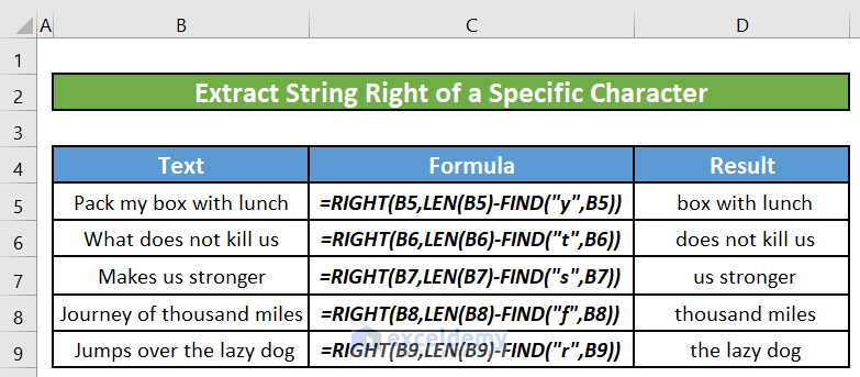
Method 5 – Extracting Characters from the Right of a Specific Character

• Scenario:
  • Suppose we have a string in cell B5, and we want to extract text to the right of a specific character (in this case, the character “y”).

• Formula:
  • In cell B5, enter the following formula:

• • • LEN(B5) calculates the total number of characters in the string (which is 22 in this case).
    • FIND(“y”, B5) calculates the position of the character “y” in the string (which is 7).
    • Subtracting LEN(B5) from FIND(“y”, B5) gives us the number of characters to the right of the character “y” (which is 15).
• Result:
  • The RIGHT function will extract the 15 characters from the end (right) of the string, starting from the character “y”.

• Repeat:
  • You can apply the same approach to other strings, selecting different characters each time.

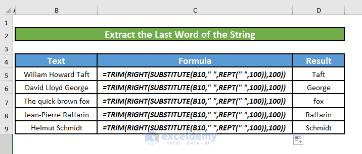
Method 6 – Finding the Last Word From the Right in Excel

• Scenario:
  • Suppose we have a text string in cell B5, and we want to extract the last word from it.

• Formula:
  • In cell B5, enter the following formula:

• • • Breakdown of the formula:
      • SUBSTITUTE(B5, ” “, REPT(” “, 100)): This part replaces all spaces in the original string with 100 spaces. It ensures that we have enough spaces to cover any word.
      • RIGHT(…): Extracts the last 100 characters from the modified string.
      • TRIM(…): Removes any extra spaces from the extracted portion, leaving only the last word.

• Result:
  • The formula will return the last word from the right in the original text string.

• Repeat:
  • You can apply the same approach to other strings.

Read More: How to Find Text in Cell in Excel

Things to Remember

• If you don’t specify a number as the second argument for the RIGHT function, it will extract the last character of the string.
• If the second argument exceeds the total length of the string, it will return the entire string.

Download Practice Workbook

You can download the practice workbook from here:

Related Articles

• How to Find If Range of Cells Contains Specific Text in Excel
• How to Check If Cell Contains Specific Text in Excel
• How to Find * Character Not as Wildcard in Excel

<< Go Back to Find in String | String Manipulation | Learn Excel