Method 1 – Use the Filter Shortcut Option Under the Data Tab to Filter Data
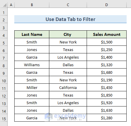
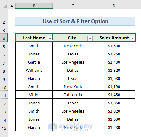
Suppose you have the following dataset.
Steps:
- Select any cell from the dataset.
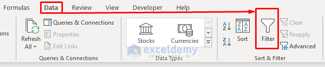
- Go to the Data Menu.
- Select the option “Filter” from the “Sort & Filter” section in the Data Ribbon.
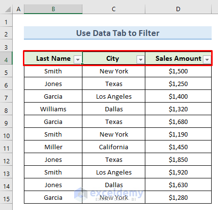
- There are now filtering drop-down icons in the headers of the dataset.
Method 2 – Filter Excel Data with ‘Sort & Filter’ Option
Steps:
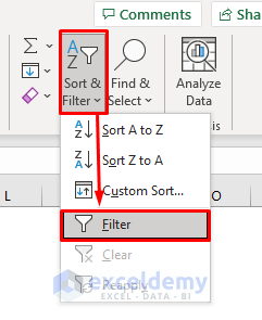
- Go to the Home tab.
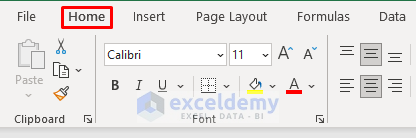
- Select the option “Sort & Filter” from the “Editing” section of the Home Ribbon.
- From the available options in the drop-down, select “Filter”.
- There are now filtering drop-down icons in the headers of the dataset.
Method 3 – Use Keyboard Shortcuts to Filter Excel Data
Seven keyboard shortcuts to quickly filter Excel data.
Example 1 – Switching On or Off the Filtering Option in Excel
Steps:
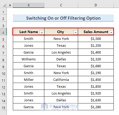
- Select any cell from the dataset.
- Press Ctrl + Shift + L at the same time.
- There are now filtering drop-down icons in the headers of the dataset.
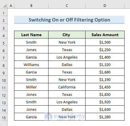
- Press Ctrl + Shift + L again and the filtering drop-down icons disappear from the header section.
Example 2 – Use Keyboard Shortcut to View the Filter Drop-Down Menu
Steps:
- Select any cell from the header.
- Press Alt + Down Arrow.
- The Filter drop-down menu for that header cell pops up.
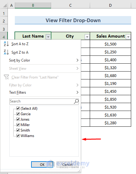
- Press the Up or Down arrow keys to select from the options.
- Press Enter.
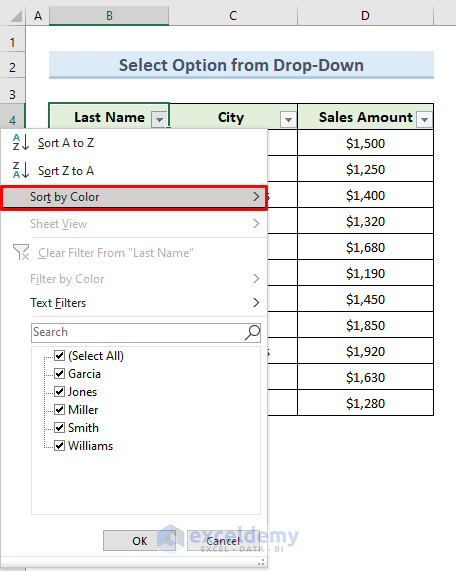
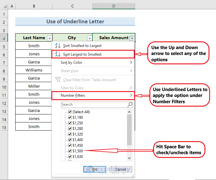
Example 3 – Use Underlined Letters to Filter Excel Data
There are many keyboard shortcuts in Excel. To make them easier to remember, Excel has underlined letters in certain menus and pop-ups. In addition, the up and down arrows and space bar can be used to navigate and select/deselect these options.
| SHORTCUT | SELECTED OPTION |
|---|---|
| Alt + Down Arrow + S | Sort Smallest to Largest or A to Z |
| Alt + Down Arrow + O | Sort Largest to Smallest or Z to A |
| Alt + Down Arrow + T | Open the submenu Sort by Color |
| Alt + Down Arrow + I | Access the submenu Filter by Color |
| Alt + Down Arrow + F | Select the submenu Date Filter |
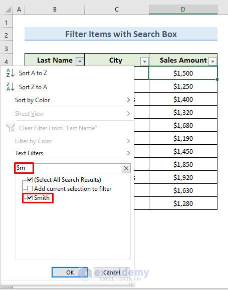
Example 4 – Filter Items with the Search Box in Excel
Steps:
- Open the filtering drop-down menu in a dataset.
- Press Alt + Down Arrow + E. This will activate the search box.
- Input text in the search box.
- Data matching that text will show below the search box.
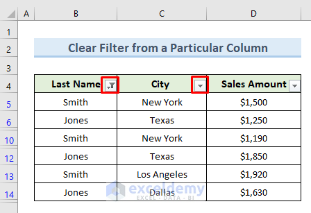
Example 5 – Clear Filter from a Particular Column of a Data Range
Steps:
- Select one of the header cells.
- Press Alt + Down Arrow + C.
- Filtering for that colum has been removed.
Example 6 – Filter Excel Data with a Custom Filter Dialogue Box
Steps:
- Select one of the header cells.
- Press Alt + Down Arrow to view the filtering drop-down menu.
- Click the F and E keys.
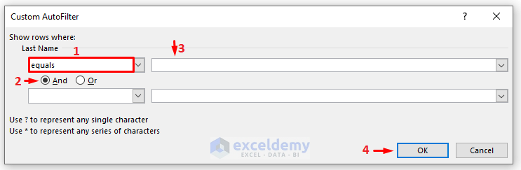
- A new dialogue box named “Custom Autofilter” will open.
- Input the desired parameters from the drop-down lists. Double check the proper And/Or option is checked.
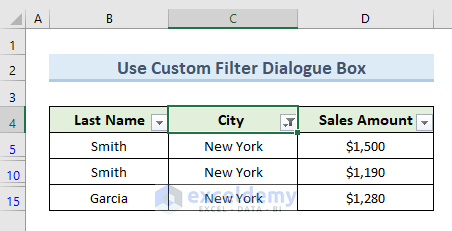
- Click OK.
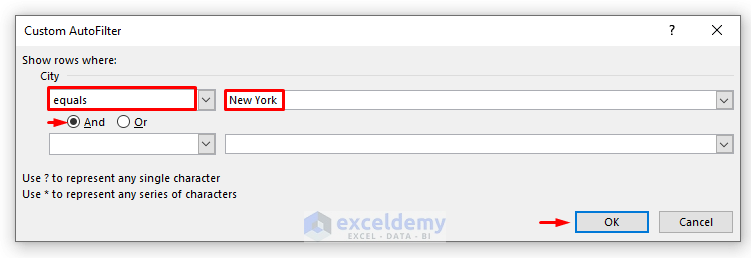
- A table with only the chosen data appears.
Example 7 – Use Keyboard Shortcuts to Filter Blank or Non-Blank Cells
Sometimes a dataset contains Blank cells as well as cells filled with data.
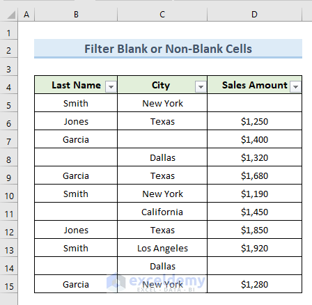
Steps:
- Select a header cell. Press Alt + Down.
- Click the F and E keys respectively to open the custom filter dialogue box.
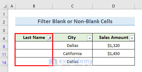
- Choose equals from the first drop-down value, but leave the second one Blank.
- Click OK.
- Any data with a blank cell in that column will show.
To search for only Non-Blank cells:
Steps:
- Select a header cell. Press Alt + Down.
- Click the F and E keys respectively to open the custom filter dialogue box.
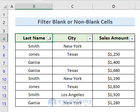
- Choose the drop-down value “not equal to” and leave the second one blank.
- Press OK.
- Only data without a blank cell in that column will show.
Things to Remember
- To apply filtering in more than one data range in a single worksheet use the Excel Table Feature.
- Use one filtering option at a time per column. For example, you can’t use a Text filter and a Color filter at the same time.
- Avoid using different kinds of data in the same column.
Download Practice Workbook
You can download the practice workbook from here.
<< Go Back to Filter in Excel | Learn Excel
Get FREE Advanced Excel Exercises with Solutions!
