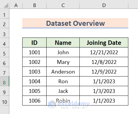
This is the sample dataset.
Method 1 – Using the Connections Function to Create an Excel Data Connection to Another Excel File
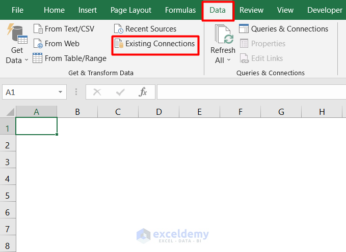
Steps:
- Open a new workbook.
- Go to the Data tab and select Existing Connections.
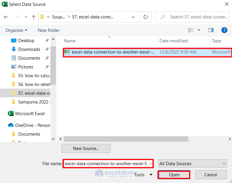
- Select Browse for More.

- Select the source file.
- Click Open.
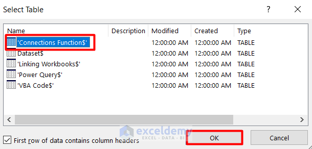
- Choose the table in the dialog box.
- Click OK.
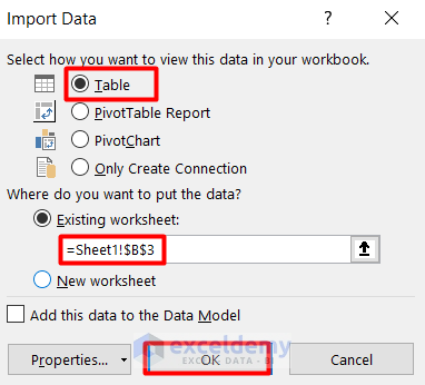
- Select Table and enter the destination in Existing Worksheet.
- Click OK.
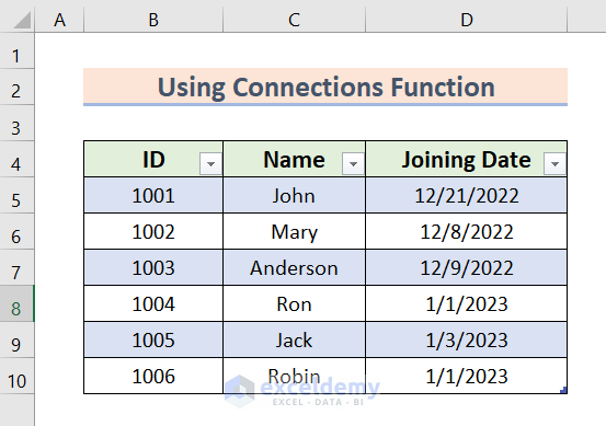
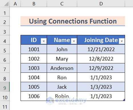
The table will be pasted:
Method 2 – Using a VBA Code to Create an Excel Data Connection
Steps:
- Press Alt + F11.
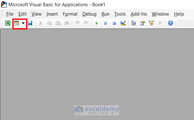
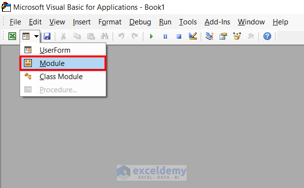
- Select the icon shown below.
- Select Module.
- Enter the following code in the module.
Sub ImportDatafromotherworksheet()
Dim ss_wkbCrntWorkBook As Workbook
Dim ss_wkbSourceBook As Workbook
Dim ss_rngSourceRange As Range
Dim ss_rngDestination As Range
Set ss_wkbCrntWorkBook = ActiveWorkbook
With Application.FileDialog(msoFileDialogOpen)
.Filters.Clear
.Filters.Add "Excel 2007-13", "*.xlsx; *.xlsm; *.xlsa"
.AllowMultiSelect = False
.Show
If .SelectedItems.Count > 0 Then
Workbooks.Open .SelectedItems(1)
Set ss_wkbSourceBook = ActiveWorkbook
Set ss_rngSourceRange = Application.InputBox(prompt:="Select source range", Title:="Source Range", Default:="A1", Type:=8)
ss_wkbCrntWorkBook.Activate
Set ss_rngDestination = Application.InputBox(prompt:="Select destination cell", Title:="Select Destination", Default:="A1", Type:=8)
ss_rngSourceRange.Copy ss_rngDestination
ss_rngDestination.CurrentRegion.EntireColumn.AutoFit
ss_wkbSourceBook.Close False
End If
End With
End Sub
Variables were declared to create a data connection to another Excel file and statements were used to apply the conditions.
- Press F5 to run the code.
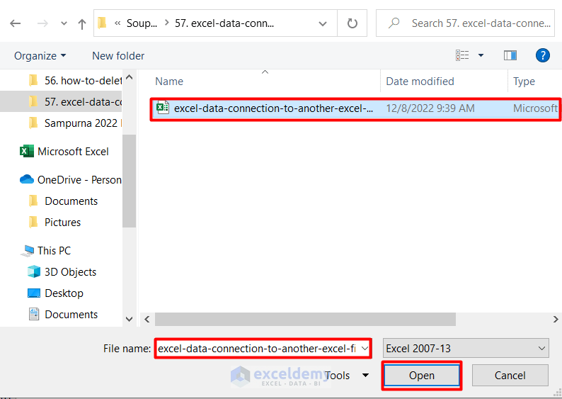
- In the dialog box, select the file.
- Click Open.
- Select the source range.
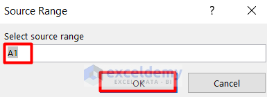
- Select the table: B4:D10.
The dialog box will show the source range:
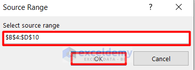
- Click OK.
- Select the destination: B4.
- Click OK.

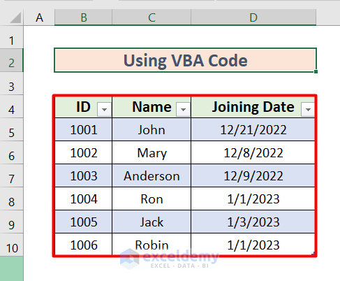
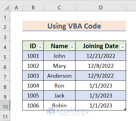
The connected data table is displayed.
Read More: Excel VBA: How to Refresh All Data Connections
Method 3 – Applying the Power Query
Steps:
- Open a new sheet.
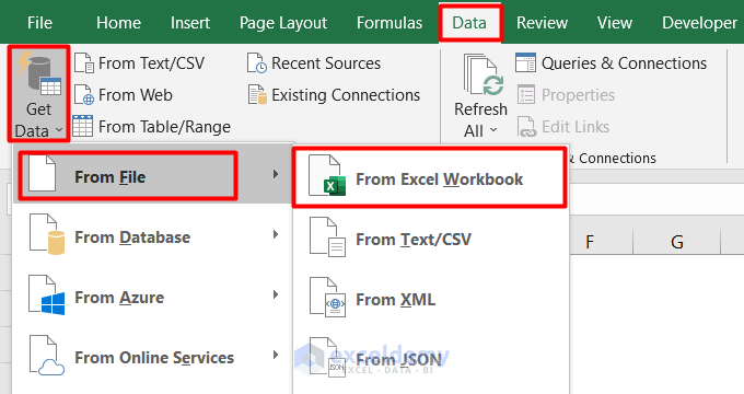
- Go to the Data tab.
- Select Get Data.
- Click From File.
- Select From Excel Workbook.
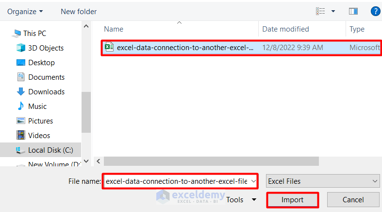
- Select the file and click Import.
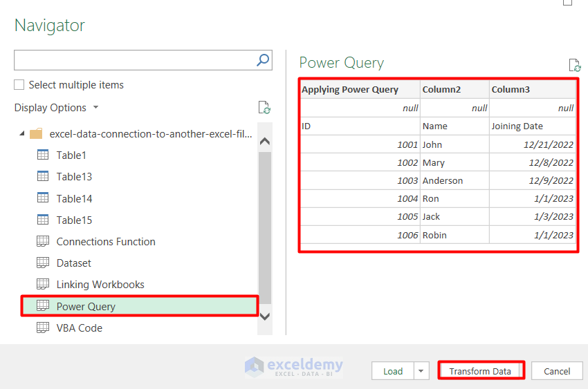
- In the Navigator panel, select Power Query.
- Click Transform Data.
- Go to the Home tab and select Remove Rows.
- Choose Remove Top Rows.
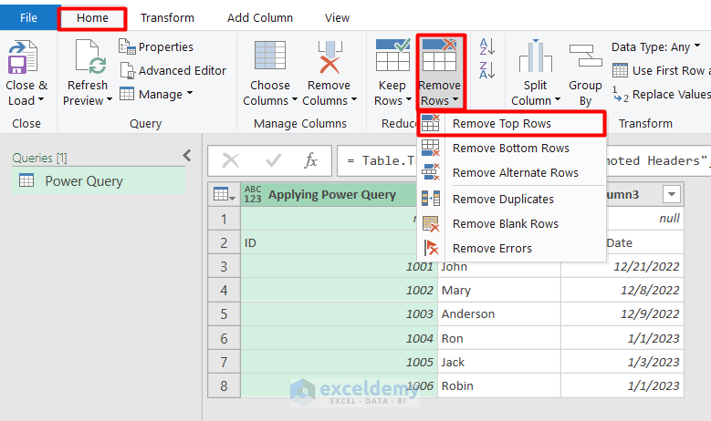
- Specify the number of rows to remove.
- Click OK.

A preview is displayed.

- Go to Transform.
- Select Use First Row as Headers.

You can see the preview in the selected area.
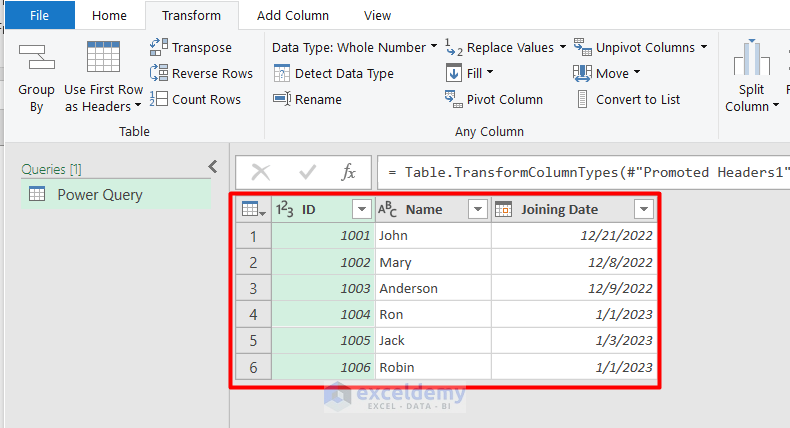
This is the output.

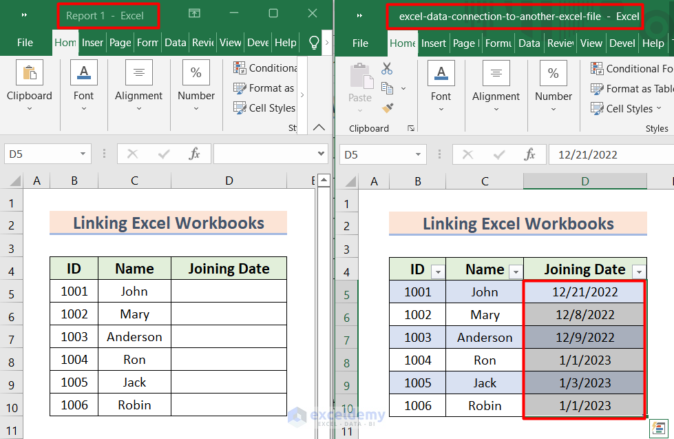
Linking Excel Workbooks for Automatic Update
Two data tables from different workbooks were used:
Steps:
- Copy the joining date in the selected area, as shown below.
- Right-click the Joining Date column in Report-1.
- Select Paste Special.

- Select Paste Link.

Joining Dates will be connected.

Read More: How to Create a Data Source in Excel
Download Practice Workbook
Download the workbook.
Related Articles
- How to Refresh Data Connection in Excel Without Opening File
- Data Connection Not Refreshing in Excel
- [Fixed!] External Data Connections Have Been Disabled in Excel
- Excel Connections vs. Queries
- Excel Queries and Connections Not Working
<< Go Back to Excel Data Connections | Importing Data in Excel | Learn Excel
Get FREE Advanced Excel Exercises with Solutions!
