How to Color Alternate Row for Merged Cells in Excel

If you work with large data sets in Microsoft Excel, you may find it helpful to format alternate rows with a different color. This can make it easier to scan the data and spot patterns or trends. You can use VBA code to apply alternative row colors for merged cells quite easily. In this article, I will show you how to alternate the row color for merged cells in Excel with ease. So, without having any further discussion, let’s begin.

How to Color Alternate Row for Merged Cells in Excel: Easy Steps

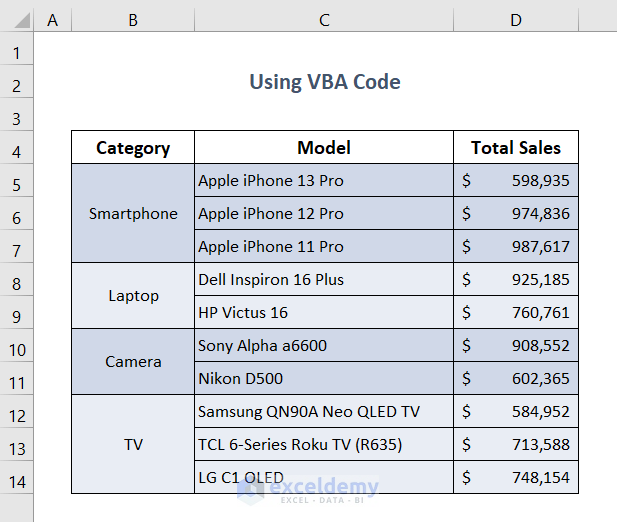
In the following dataset, the left-most column, Category has various product category names. There I used the Merge Cells command to merge consecutive rows. The merging of rows doesn’t have any particular pattern in row numbers. I will use this dataset to show you apply alternative the row color in Excel.

Step-1: Open Visual Basic Editor

I will use a VBA code to apply the alternative row color scheme for merged cells in Excel. To use the VBA code, you need to open the Visual Basic Editor first.

For that,

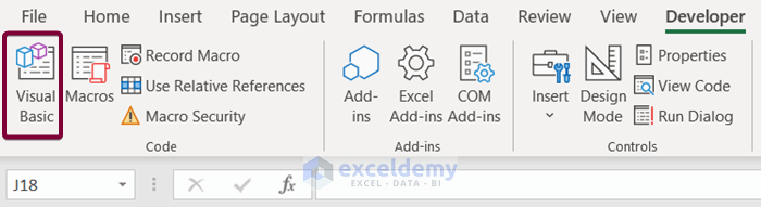
❶ Go to the Developer tab in the ribbon.

❷ Now click on the Visual Basic command in the Code group.

This will open the Visual Basic Editor straightway.

Alternatively, you can press the ALT + F11 keys to open the Visual Basic Editor.

Step-2: Insert VBA Code in a New Module

Now you need to open a new module to insert the VBA code. To open a new Module,

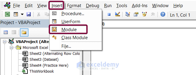
❶ Go to the Insert tab.

❷ Select the Module command from the drop-down list.

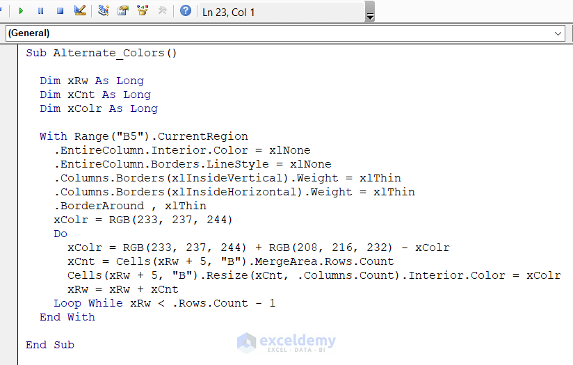
❸ Now copy the following VBA code.

Sub Alternate_Colors()

  Dim xRw As Long
  Dim xCnt As Long
  Dim xColr As Long

  With Range("B5").CurrentRegion
    .EntireColumn.Interior.Color = xlNone
    .EntireColumn.Borders.LineStyle = xlNone
    .Columns.Borders(xlInsideVertical).Weight = xlThin
    .Columns.Borders(xlInsideHorizontal).Weight = xlThin
    .BorderAround , xlThin
    xColr = RGB(233, 237, 244)
    Do
      xColr = RGB(233, 237, 244) + RGB(208, 216, 232) - xColr
      xCnt = Cells(xRw + 5, "B").MergeArea.Rows.Count
      Cells(xRw + 5, "B").Resize(xCnt, .Columns.Count).Interior.Color = xColr
      xRw = xRw + xCnt
    Loop While xRw < .Rows.Count - 1
  End With

End Sub

❹ Paste it to the newly opened module.

Step-3: Save Workbook as Macro-Enabled Workbook

To save the workbook with the VBA code,

❶ Go to the File tab in the ribbon.

❷ Then select the Save command.

Or you can press the CTRL + S keys together.

❸ Next click No in the pop-up dialog box to proceed with the VBA code.

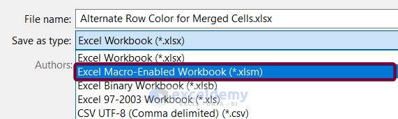
❹ Now select Excel Macro-Enabled Workbook (*.xlsm) option in the Save as type drop-down.

Step-4: Run VBA Code

Now all you need to do is run the code. To run the VBA code,

❶ Go to the Developer tab.

❷ Select the Macros command in the Code group.

Or you can press the ALT + F8 keys to open the Macro dialog box.

❸ Next, click on the Run button in the Macro dialog box.

Thus, the VBA code will run. This code will alternate the row color for the merged cells just like in the following picture.

Practice Section

You will get an Excel sheet like the following screenshot, at the end of the provided Excel file where you can practice all the topics discussed in this article.

Download Practice Workbook

You can download the Excel file from the following link and practice along with it.

Conclusion

I have discussed steps to alternate row colors for merged cells in Excel. Please don’t hesitate to ask any questions in the comment section below. We will try to respond to all the relevant queries ASAP.

Related Articles

• How to Alternate Row Color Based on Group in Excel
• How to Color Alternate Row Based on Cell Value in Excel
• How to Alternate Row Colors in Excel Without Table

<< Go Back to Alternating Row Colors | Highlight Row | Highlight in Excel | Learn Excel