How to Change Date Alignment in Excel: 8 Simple Methods

Method 1 – Change Date Alignment with Text to Columns Feature

STEPS:

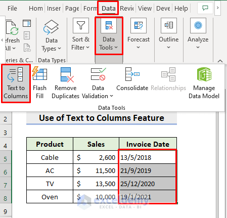
• Select the date range D5:D8.
• Go to Data > Data Tools > Text to Columns.

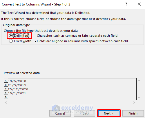
• A dialog box will pop out.
• Select Delimited and press Next.

• Press Next in the step 2 dialog box.
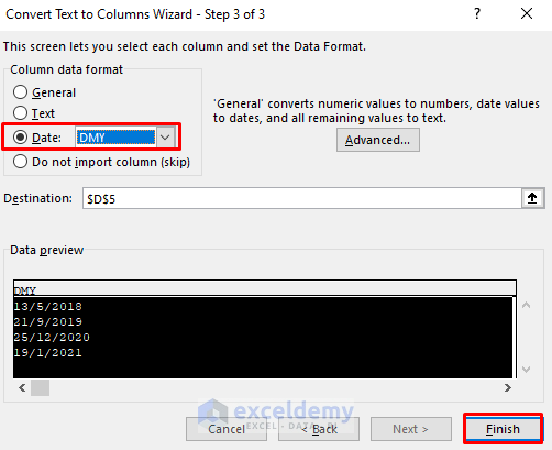
• In step 3, choose Date and DMY from the drop-down options.
• Press Finish.

• You’ll see the accurate date alignment.

Method 2 – Insert VALUE Function to Align Date in Excel

STEPS:

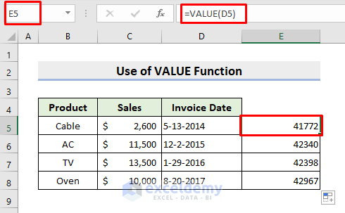
• Select cell E5.
• Type the formula:

• Press Enter and use AutoFill to get all the results.

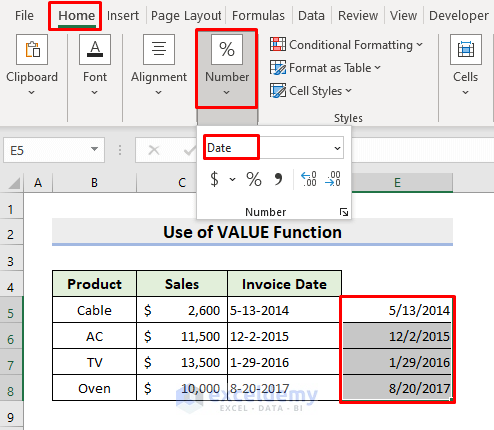
• Select the range E5:E8.
• Choose the Date format from the Number drop-down in the Home tab.
• Return the desired output.

Method 3 – Align Date Using DATEVALUE Function

STEPS:

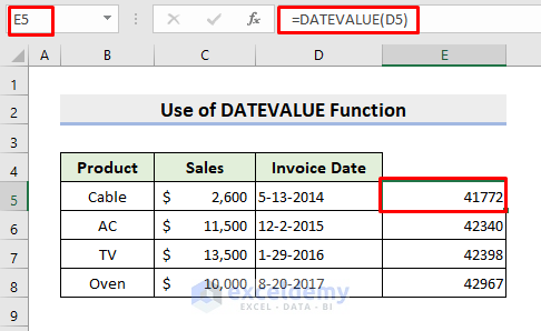
• Click cell E5.
• Input the formula:

• Press Enter.
• Apply AutoFill.

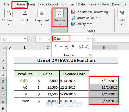
• Select the range and choose Number > Date under the Home tab.
• Get the precise date alignment.

Method 4 – Set Date Alignment with Excel Find & Replace Feature

STEPS:

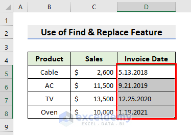
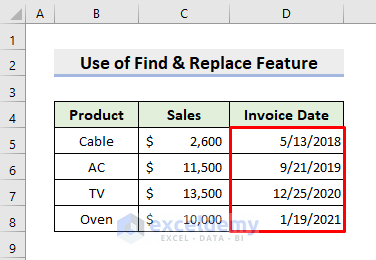
• Select the range D5:D8 at first.

• Press the Ctrl and H keys together.
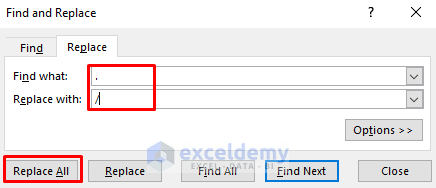
• The Find and Replace box will emerge.
• Insert in Find what and / in Replace with.
• Click Replace All.

• Return the worksheet after making the required corrections.
• You can change the date alignment.

Method 5 – Combine VALUE and SUBSTITUTE Functions for Fixing Date Alignment

STEPS:

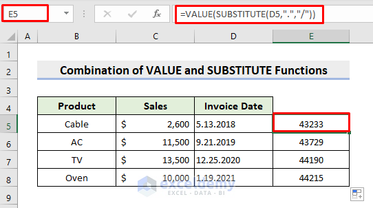
• Choose cell E5.
• Insert the formula:

• Press Enter and use AutoFill.
• The SUBSTITUTE function replaces period (.) with / in cell D5.
• The VALUE function converts it to a number.

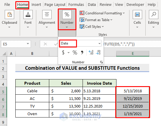
• Select the range E5:E8.
• Choose Number > Date as the number format.
• Perfectly aligned dates will appear.

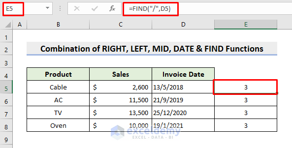
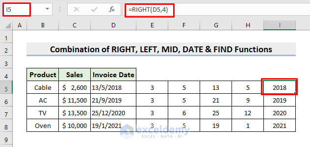
Method 6 – Align Date with Combination of RIGHT, LEFT, MID, DATE & FIND Functions

STEPS:

• Click cell E5.
• Type the formula:

• Press Enter and apply AutoFill.

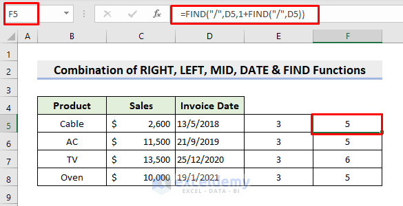
• In cell F5, input:

• Hit Enter.
• This formula looks for the second / symbol and returns its position.
• Use AutoFill.

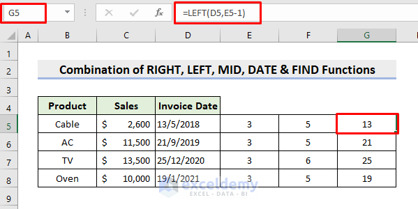
• Choose cell G5 to insert the formula:

• Click Enter.
• Return other results by using AutoFill.

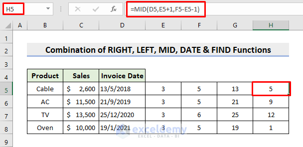
• In the H5 cell, insert:

• Return output by pressing Enter.
• Use AutoFill.

• Choose I5 for the formula:

• Click Enter and apply AutoFill.

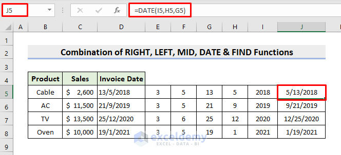
• In cell J5, insert:

• This formula will return accurate date alignment after pressing Enter.
• Apply AutoFill to get other results.

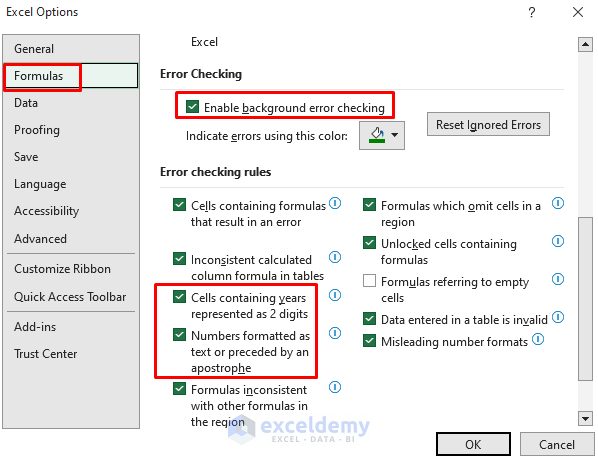
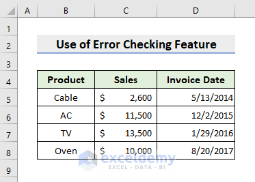
Method 7 – Apply Excel Error Checking Feature to Change Date Alignment

STEPS:

• Go to File > Options.
• Make sure you check the boxes for the marked options in the Formulas tab.
• See the below picture for a better understanding.

• You have the year in only 2 digits, Excel will show a green shade on the upper-left side of the cell.
• Select the cell, and you’ll see the warning symbol.
• Click the drop-down symbol and choose Convert XX to 20XX.

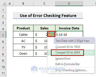
• It’ll return the date in perfect alignment.

Method 8 – Align Date with Excel Power Query

STEPS:

• Select the range B4:D8.
• Go to Data > Get & Transform Data > From Table/Range.

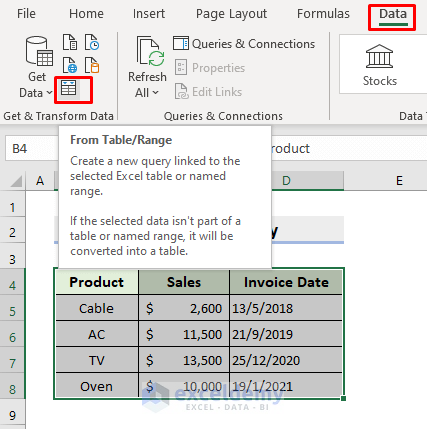
• A dialog box will appear and press OK.
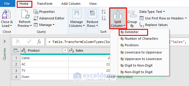
• Select the Date column.
• Click Split Column > By Delimiter.

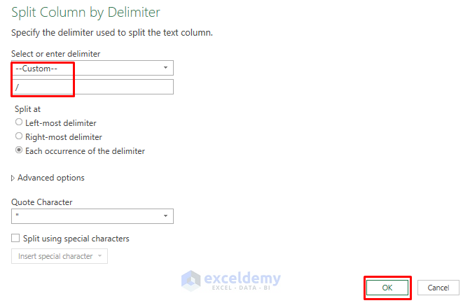
• In the pop-out dialog box, type / in the Custom delimiter.
• Press OK.

• The column will be split into 3 columns.
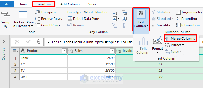
• Select the month, day, and year columns at the same time.
• Click Transform > Text Column > Merge Columns.

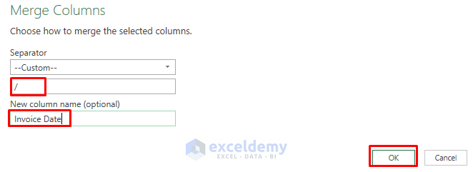
• In the dialog box, type / in the custom separator.
• Input the new column name.
• Press OK.

• Click the entire merged column and choose Data Type > Date.
• Press Close & Load.

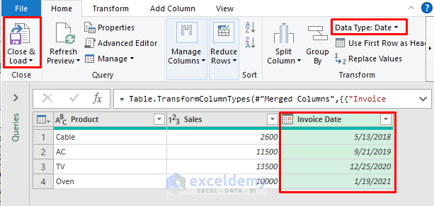
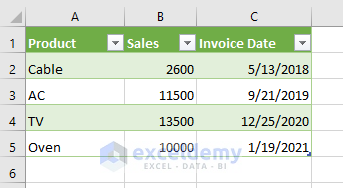
• You’ll get a new Excel worksheet with the required date alignment.

Download Practice Workbook

Download the following workbook to practice by yourself.

Related Articles