Fix Excel Date Not Formatting Correctly (8 Quick Solutions)

Here’s an overview of fixing the date format in Excel. You can use the Text to Columns feature to extract and format dates from cells.

Fix 1 – Converting the Text String to an Excel Date Format Correctly

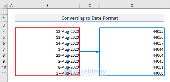
When copying dates from one range to the other, you may get integer or decimal values instead of dates. This is due to Excel saving dates as numbers.

Steps:

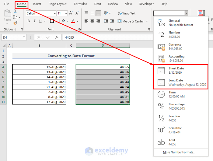
• Select the range of cells containing the number values that have to be turned into date format.
• Under the Home tab and from the Number group of commands, click on the drop-down.
• You’ll see two types of date format there: Short Date and Long Date.
• Select any one of these two formats.

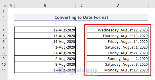
• Here’s the result.

Fix 2 – Customizing the Date Formatting Correctly in Excel

Steps:

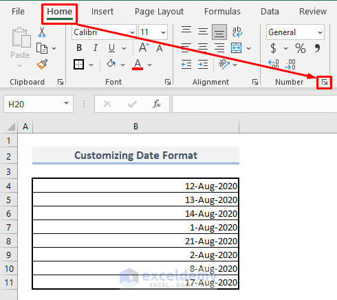
• Under the Home ribbon, open the Cell Format dialogue box from the Number group of commands by pressing on the arrow at the corner.

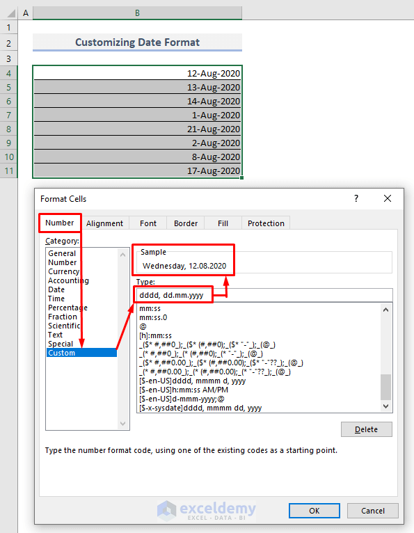
• Select Custom under the Number tab.
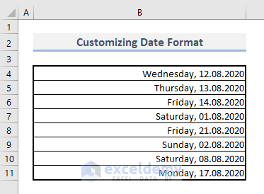
• We want to see the date format as ‘Wednesday, 12.08.2020’. Under the Type option, we wrote:

dddd, dd.mm.yyy

• You’ll be shown a preview under the Sample bar.
• Press OK.

• Here are the results.

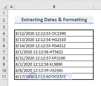
Fix 3 – Extracting Dates from Text by Using the Column Wizard

If the strings contain values other than dates, then you can’t convert them directly via Format Cells.

Steps:

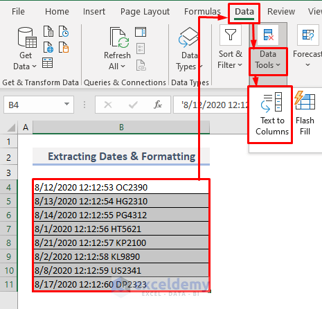
• Select the entire range of cells containing the texts with dates.
• From the Data tab, choose the Text to Columns option from the Data Tools drop-down..

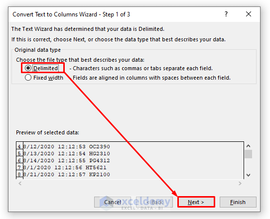
• You’ll get a Text to Columns wizard.
• Select Delimited and press Next.

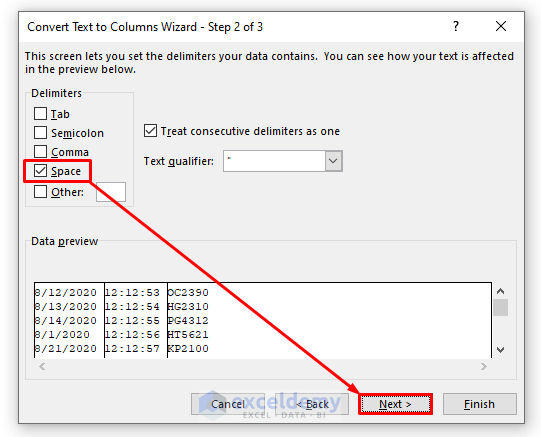
• Check Space as the delimiter since the sample text data contains spaces among them.

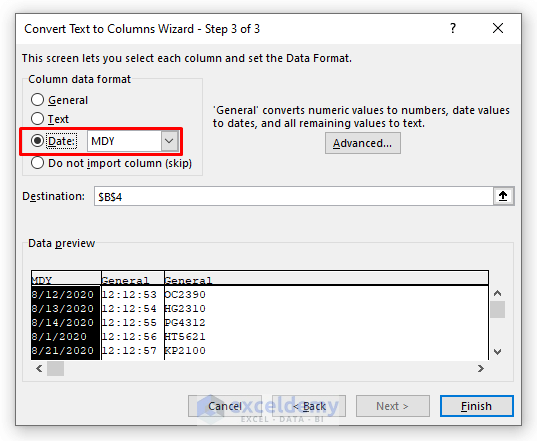
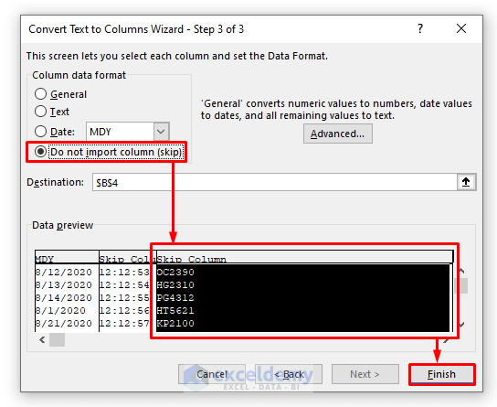
• You’ll get a preview of the resulting columns. Select Date as the Column Data Format.
• The dates in the texts are in MM/DD/YYYY format so select MDY format from the Date drop-down.

• Click on the second column now in the Data Preview section.
• Select Do not import column(skip) radio button for Column Data Format.

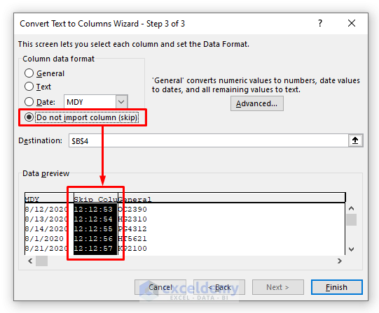
• Click on the third column.
• Select Do not import column(skip) for Column Data Format for the third column, too.
• Press Finish.

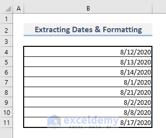
• You’ll get a range of cells that contains dates.

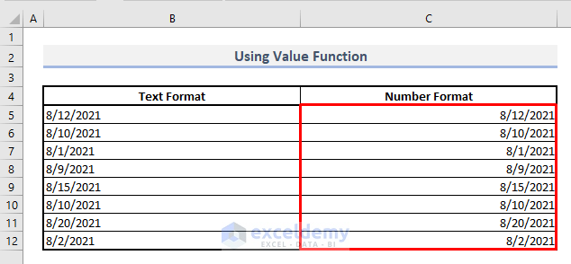
Fox 4 – Using the VALUE Function to Fix the Date Format

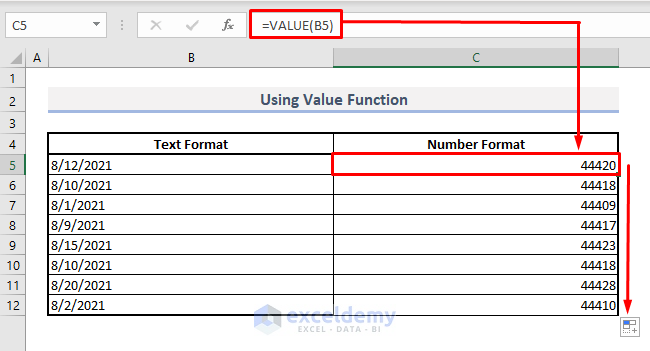
In Column B, we have dates with text format though they look like in the exact date format.

Steps:

• Select Cell C5 and insert the following:

• Press Enter and the function will return numbers.
• Use the Fill Handle now to autofill the entire Column C.
• The text format has just turned into number format.

• Select the range containing the results.
• Under the Number group of commands in the Home tab, select Short or Long Date format.

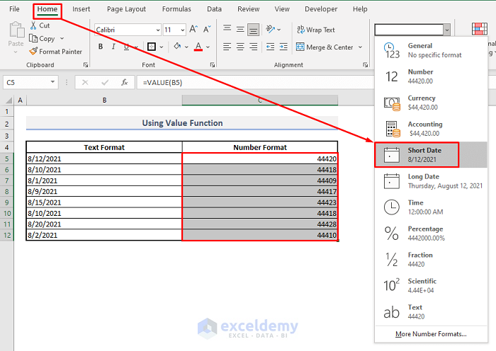
• The dates will be displayed in a proper format in Column C.

Read More: How to Convert a Date to dd/mm/yyyy hh:mm:ss Format in Excel

Fix 5 – Inserting the DATEVALUE Function to Fix the Date Format in Excel

If other strings except date or time exist in the cell, the DATEVALUE function cannot recognize the date or time data in the cell and will return as #VALUE! error. The syntax of this DATEVALUE function is:

=DATEVALUE(date_text)

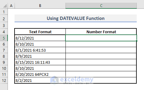
Steps:

• Select Cell C5 and insert:

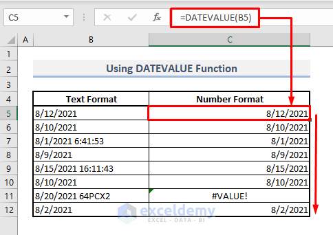
• Press Enter and use the Fill Handle to autofill other cells in Column C.
• The text values will turn into number format. Change the format of those numbers into date format.
• We get an error cell due to a string that’s not a date in the source. Fix that manually or using another option.

The basic difference between uses of VALUE and DATEVALUE functions is DATEVALUE function extracts only dates from a combination of date and number from a cell. But the VALUE function searches for numbers only from a text string no matter it represents a date or time value.

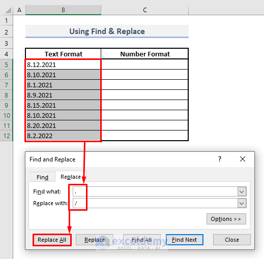
Fix 6 – Applying Find and Replace to Convert Text into Dates

If the dates include Dots(.) instead of Obliques(/) as the separators, the VALUE or DATEVALUE function will not be able to recognize date value from a text string.

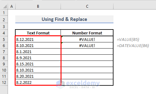
Steps:

• Select the text data containing dates.
• Press Ctrl + H to open the Find and Replace dialog box.
• Input a Dot(.) for Find What and a Forward Slash(/) for Replace With.
• Press Replace All.

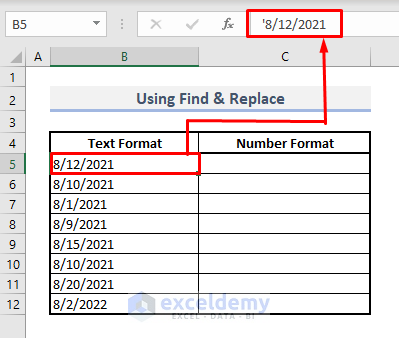
• All date values in Column B will get slashes as separators.

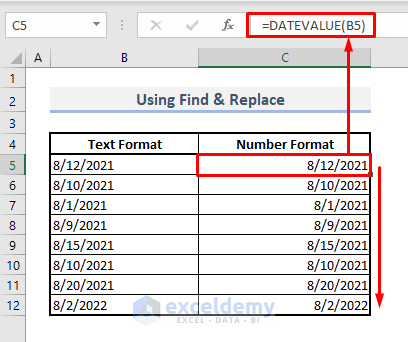
• In Cell C5, use the DATEVALUE function to convert the text format into a number format that will represent dates.

• Use Fill Handle to fill down the rest of the cells and you’ll find the dates in accurate format.

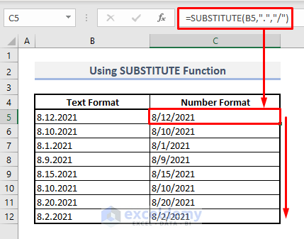
Fox 7 – Using the SUBSTITUTE Function for Formatting Dates

Another way to remove improper date separators is via the SUBSTITUTE function.

=SUBSTITUTE(text, old_text, new_text, [instance_num]

Steps:

• In Cell C5, insert the following:

• Press Enter and autofill the entire Column C with the Fill Handle.
• You’ll get the values with the proper date formatting.

Fix 8 – Using the Error-Checking Option to Fix Date Format

The cells containing dates in an improper format can show errors that you can find by clicking on the yellow icon with the exclamation sign.

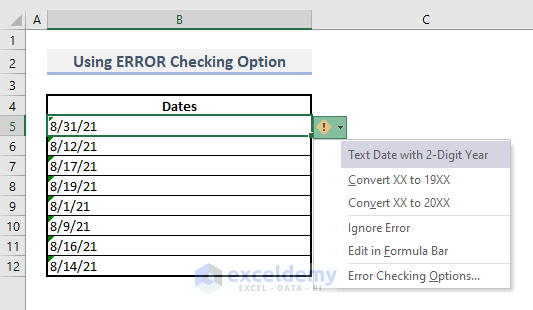
• Select the option that will convert the 2-digit year to the 4-digit year with the 20XX year format. If the years in your data represent 1900-1999, choose 19XX.

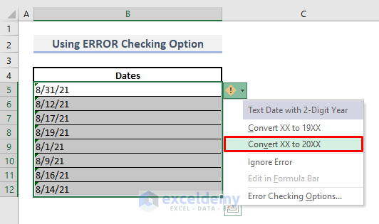
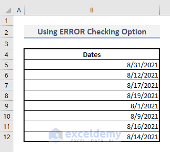
• Excel will automatically fix the values.

Things to Remember

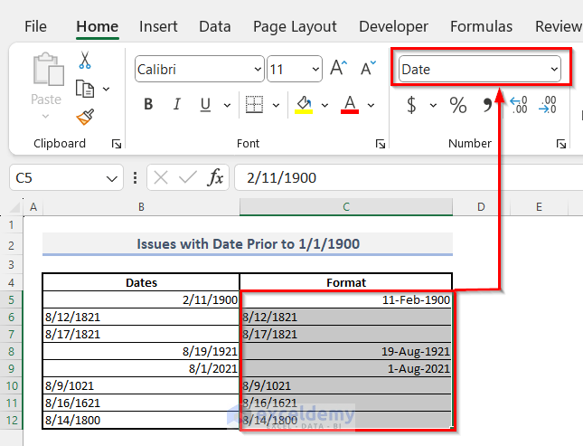
Excel stores the date values as numbers. By default, this counting starts from 1st January of 1900. However, the program doesn’t recognize dates before that as valid inputs for the date format. If you want to calculate using those dates, one of the options is to add 1,000 years to the date and use that value for calculations, then use a custom format to display it.

Download the Practice Workbook

Related Articles

• How to Change Default Date Format from US to UK in Excel
• How to Change Date Alignment in Excel

<< Go Back to Date Format | Number Format | Learn Excel