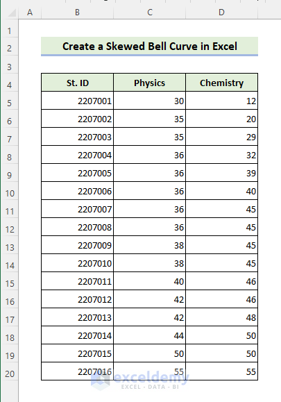
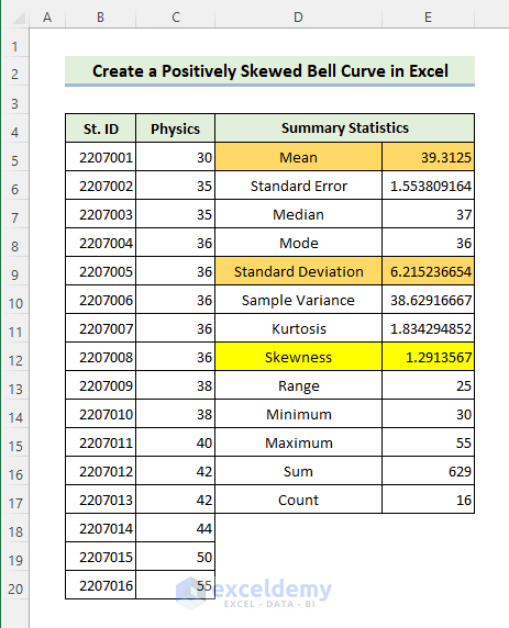
For illustration, we will use the following dataset to create a bell curve to compare the results.
Step 1 – Generate a Summary Statistics
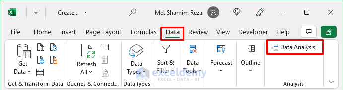
- Select Data >> Data Analysis.
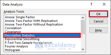
- Select Descriptive Statistics and click OK.
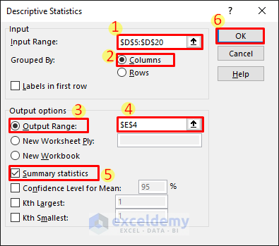
- Enter D5:D20 (Physics) for Input Range.
- Select the radio button for Columns.
- Select the radio button for Output Range.
- Enter E4 for the output range.
- Check the Summary statistics.
- Click OK.
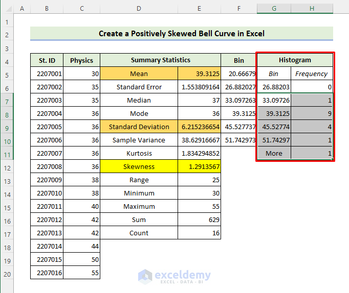
- It will output the following result. You can see that the Skewness is 1.29 indicating a highly positively skewed dataset. We will need the Mean and Standard Deviation from this table to create the skewed bell curve.
Step 2 – Create a Bin Range
- Enter the following formula in Cell F5.
=$E$5-3*$E$9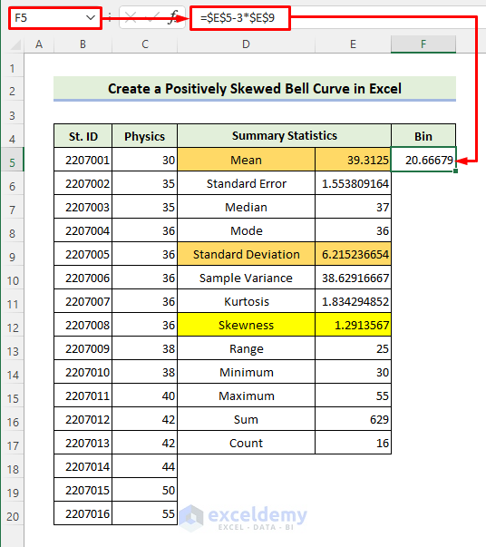
- Apply the following formula in cell F6 and drag the fill handle icon up to cell F10.
=F5+$E$9
Step 3 – Generate a Histogram
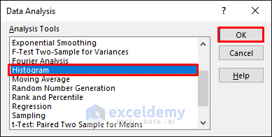
- Select Data >> Data Analysis.
- Select Histogram and click OK.
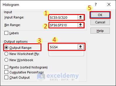
- Enter C5:C20 and F6:F10 for the Input Range and the Bin Range.
- Select the radio button for Output Range.
- Enter G4 for the output range.
- Click OK.
- You will get the following result. Select range G7:H11 from the histogram table.
Step 4 – Insert Skewed Bell Curve
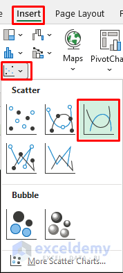
- Select Insert >> Insert Scatter (X, Y) or Bubble Chart >> Scatter with Smooth Lines.
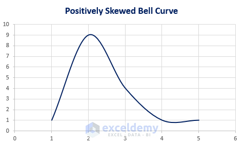
- You will get the desired skewed bell curve as shown in the following image.
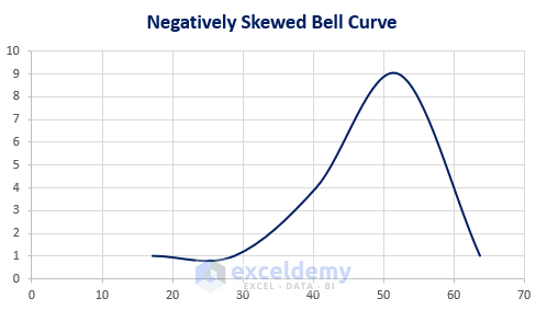
- Repeat the same procedures for the other set of data (Chemistry). You will get the following result.
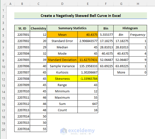
- Insert a Scatter Chart with Smooth Lines as earlier. You will get the following result.
Read More: Create a Bell Curve with Mean and Standard Deviation in Excel
Things to Remember
- You can use the SKEW function in Excel to find the skewness of a dataset.
- You must use relative and absolute references correctly in your formulas to avoid errors.
Related Articles
<< Go Back to Bell Curve in Excel | Excel for Statistics | Learn Excel
Get FREE Advanced Excel Exercises with Solutions!

Hi! Thanks for the post! very usefull for me. Learned something new.
There is a little mistake in:
Next, enter D5:D20 (Physics) for Input Range. Then, mark the radio button for Columns. Next, select the radio button for Output Range. Now, enter E4 for the output range. After that, check the Summary Statistics. Then, click OK.
Here: Next, enter D5:D20 (Physics) for Input Range. It’s “C”5 and not “D” column.
Keep the good blog! Thanxs
Hello ERICH NAGY
I appreciate your time in reading the article. I’m delighted you found the information helpful and learnt something new. Your attention to detail is really appreciated, and you are correct. The appropriate range should be the C5:C20 range instead of D5:D20. An immediate correction will be made. Once again, We appreciate your comments and support. Continue reading our blog, and we aim to offer you further helpful information soon.
Regards
Lutfor Rahman Shimanto (ExcelDemy Team)
Thank you so much I was struggling with my project and you have helped me complete it.
THANK YOUUUUUUU
Dear Vivasvan,
You are most welcome. It’s great to know that our article helped you to complete your project.
Regards
Shamima Sultana
Project Manager | ExcelDemy