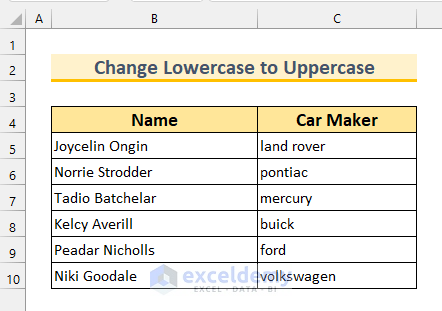
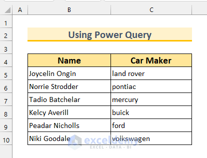
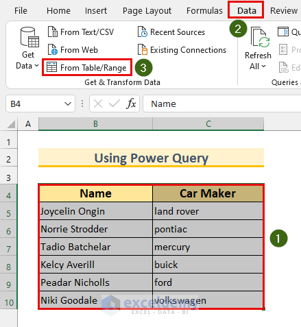
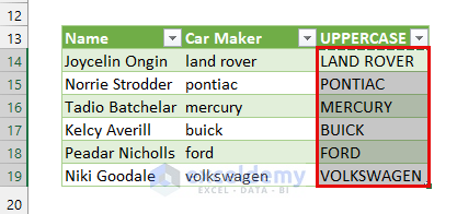
We have a dataset containing two columns, Name and Car Maker. We’ll transform the values in the Car Maker column into uppercase.
How to Change Lowercase to Uppercase in Excel: 6 Ways
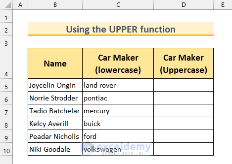
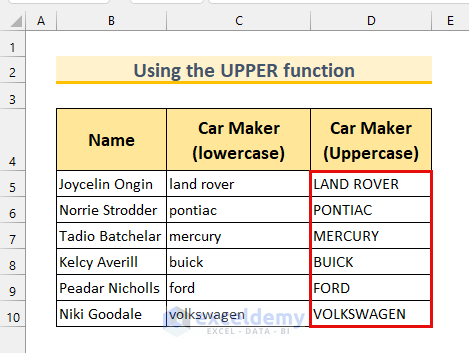
Method 1 – Using the UPPER Function to Change Lowercase to Uppercase in Excel
We’ll make a new column D to store the results of the conversion.
Steps:
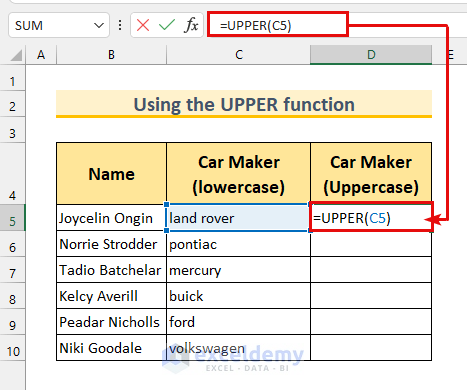
- Use the following formula in cell D5.
=UPPER(C5)The UPPER function returns the value of a cell that contains text in uppercase.
- Press Enter.
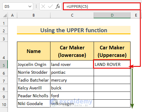
- Use the Fill Handle to AutoFill the formula.
Read More: How to Change Case in Excel Sheet
Method 2 – Applying Flash Fill to Change Lowercase to Uppercase in Excel
Steps:
- Type the first converted value of the Car Maker column in cell D5 in uppercase to make a pattern.
- Start typing the second value in D6. You’ll get a grey text box.
- That box is the Flash Fill feature with Excel’s suggestion on filling in the text.
- Press Enter.
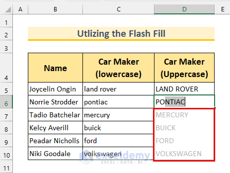
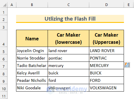
- Flash Fill automatically fills in all applicable cells that it can find.
Method 3 – Change Lowercase to Uppercase in Excel via Power Query
We’ll replace the lowercase values from the range C5:C10 to uppercase.
Steps:
- Select the cell range B4:C10.
- From the Data tab, select From Table/Range.
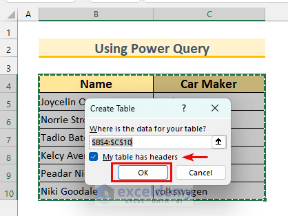
- The Create Table dialog box will appear. Make sure My table has headers is checked.
- Click on OK.
- The Power Query Editor window will open.
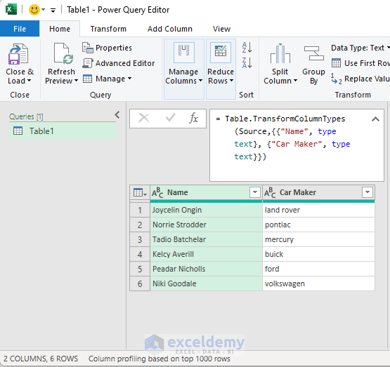
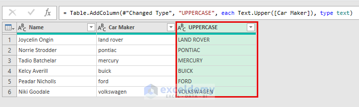
- Select the Car Maker column.
- From the Add Column tab, go to Format and select UPPERCASE.
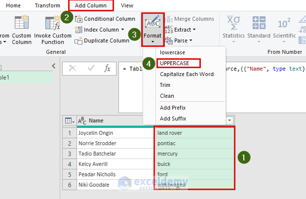
- You’ll get another column with uppercase values.
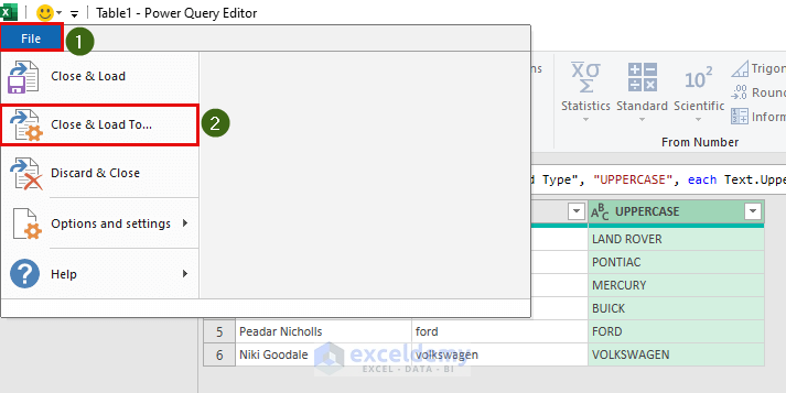
- From File, select Close & Load To…
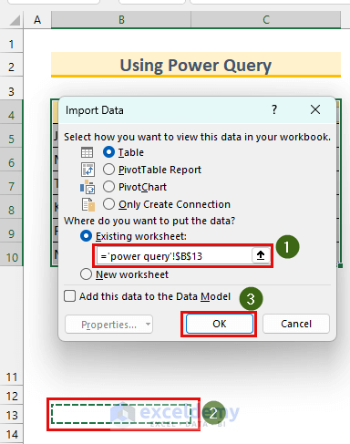
- The Import Data dialog box will appear.
- Check Existing worksheet and pick the location as cell B13.
- Press OK.
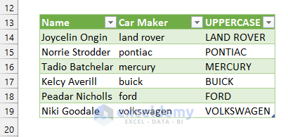
- This imports the Power Query table into the existing sheet but in a separate range.
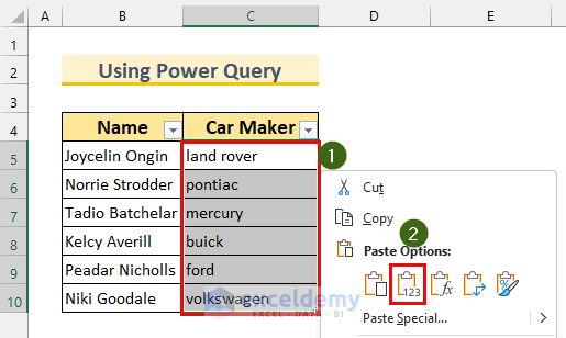
- Copy all the uppercase values from the new table.
- Right-click on the cell range C5:C10.
- From Paste Options, select Values.
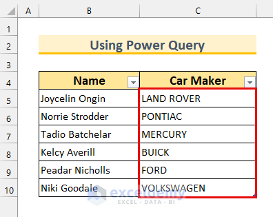
- Here’s the result.
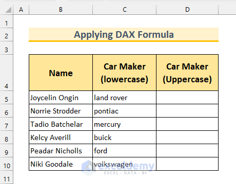
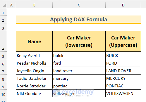
Method 4 – Implementing a DAX Formula to Change Lowercase to Uppercase in Excel
We’ll use a helper column D to store results.
Steps:
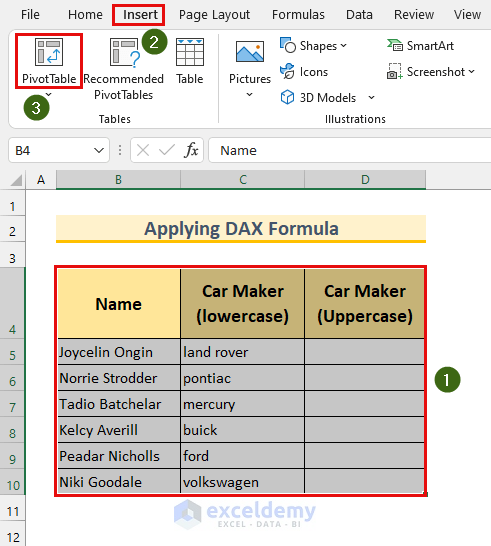
- Select the full dataset.
- From the Insert tab, select PivotTable.
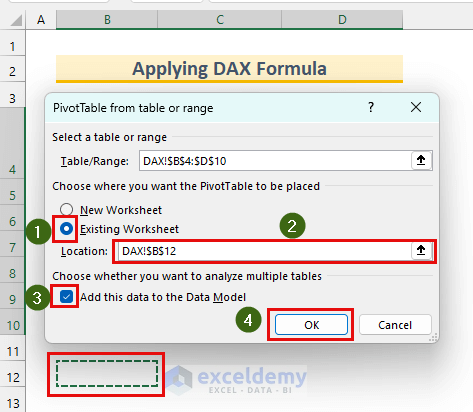
- A dialog box will appear.
- Click on Existing Worksheet and pick the Location as cell B12.
- Check Add this data to the Data Model.
- Click on OK.
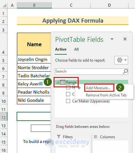
- You’ll see the PivotTable Fields option.
- Right-click on Range, then select Add Measure…
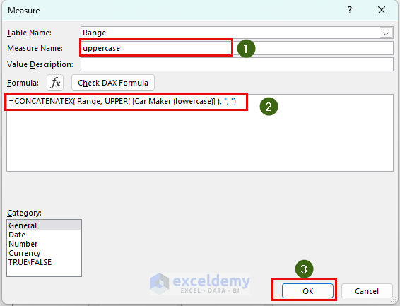
- The Measure dialog box will appear.
- Type anything in the Measure Name: box. We’ve typed “uppercase.”
- Use the following formula in the formula box.
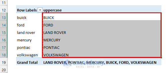
=CONCATENATEX( Range, UPPER( [Car Maker (lowercase)] ), ", ")We’re using the CONCATENATEX function from DAX and the UPPER function. The Range is our table. Finally, we’re joining the values with a comma in the Grand Total section. You can skip that comma part if you want:
=CONCATENATEX( Range, UPPER( [Car Maker (lowercase)] ))- Click on OK.
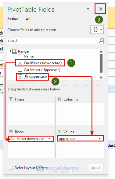
- Bring Car Maker (lowercase) to Rows and uppercase to Values by dragging with the mouse.
- Click on X to close that window.
- We can see the values are transformed into uppercase.
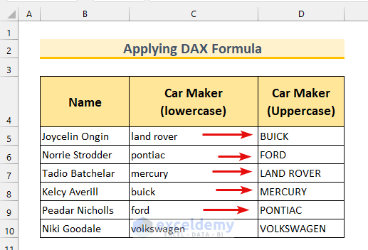
- Copy the values.
- Paste those values in cells D5:D10.
- The values were sorted automatically when the DAX formula was used.
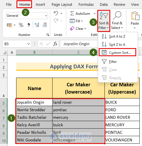
- Select the cell range B5:C10.
- From the Home tab, go to Sort & Filter and select Custom Sort…
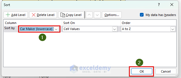
- The Sort dialog box will appear.
- For Sort by, select Car Maker (lowercase).
- Press OK.
- This sorts the original dataset to match the results.
Read More: How to Change Lowercase to Uppercase with Formula in Excel
Method 5 – Using VBA to Change Lowercase to Uppercase in Excel (Requires Range Pre-Selection)
Steps:
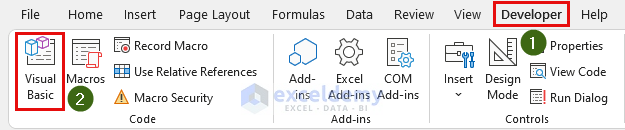
- From the Developer tab, select Visual Basic. This will bring up the Visual Basic window.
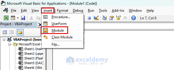
- From Insert, click on Module.
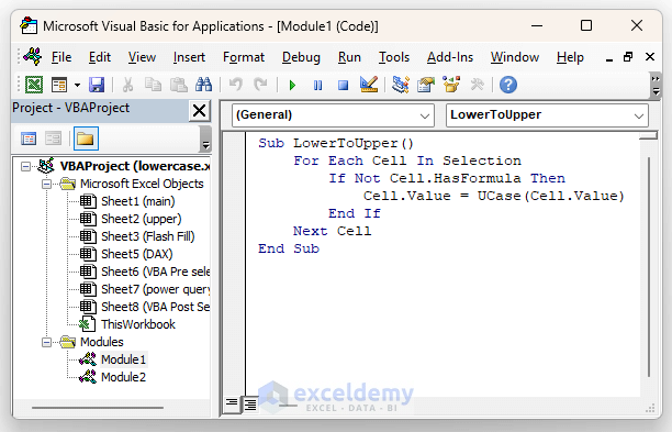
- Paste the following code into the Module.
Sub LowerToUpper()
    For Each Cell In Selection
        If Not Cell.HasFormula Then
            Cell.Value = UCase(Cell.Value)
        End If
    Next Cell
End Sub
We’re calling our Sub as LowerToUpper. It has no arguments. The code will check if the selected cell has any formula using the IF statement. If there is no formula, then the UCASE function will change the values into uppercase. A For loop will check the selection one by one.
- Save the Module and close the window.
- Select the cell range C5:C10.
- From the Developer tab, select Macros.
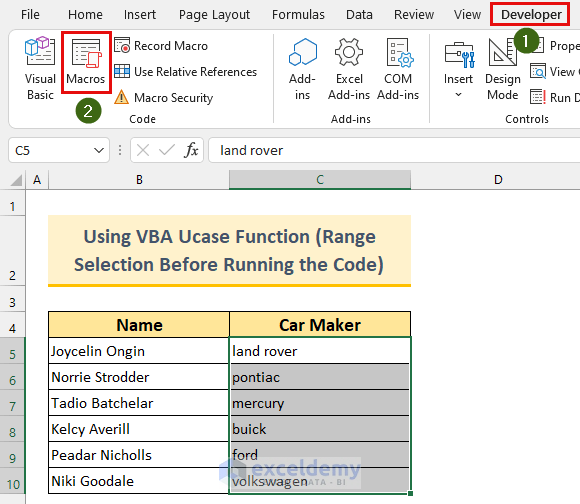
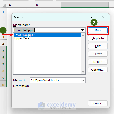
- The Macro dialog box will appear.
- Select LowerToUpper.
- Click on Run.
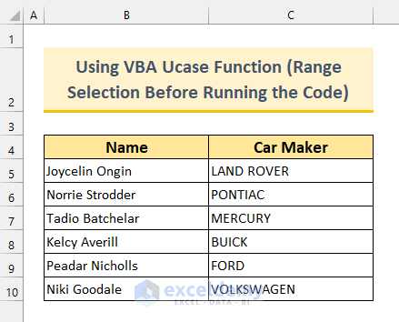
- We’ll get the uppercase values.
Read More: How to Change Case for Entire Column in Excel
Method 6 – Change Lowercase to Uppercase Using VBA in Excel (With an Input Dialog)
Steps:
- Bring up the Module window as shown in method 5.
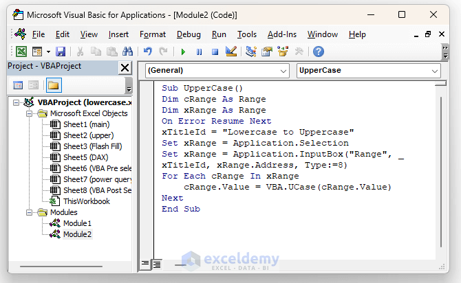
- Copy and paste the following code into the Module.
Sub UpperCase()
Dim cRange As Range
Dim xRange As Range
On Error Resume Next
xTitleId = "Lowercase to Uppercase"
Set xRange = Application.Selection
Set xRange = Application.InputBox("Range", xTitleId, xRange.Address, Type:=8)
For Each cRange In xRange
    cRange.Value = VBA.UCase(cRange.Value)
Next
End Sub
We’re defining two variables, cRange and xRange as Range. We used the Set statement to select the Range through a InputBox via Application.Selection. We set the InputBox title as “Lowercase to Uppercase”. It asks for a cell range from the user. The UCASE function will change the range to uppercase.
- Save the Module and close the window.
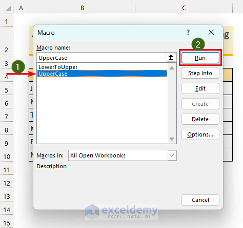
- Bring up the Macro dialog box as shown in method 5.
- Select UpperCase.
- Click on Run.
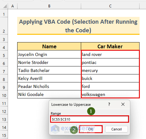
- A dialog box will ask to select a cell range. Select the cell range C5:C10.
- Press OK.
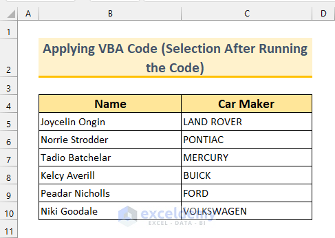
- Here are the results.
Read More: Excel VBA to Capitalize First Letter of Each Word
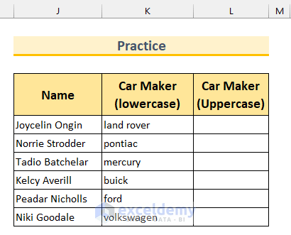
Practice Section
We’ve provided a practice dataset for each method in our Excel file.
Download the Practice Workbook
Related Articles
- How to Capitalize First Letter of Each Word in Excel
- Change Upper Case to Lower Case in Excel
- How to Make First Letter of Sentence Capital in Excel
- How to Change Sentence Case in Excel
- How to Change Lowercase to Uppercase in Excel Without Formula
<< Go Back to Change Case | Text Formatting | Learn Excel
Get FREE Advanced Excel Exercises with Solutions!
