How to Calculate Variance Using Pivot Table in Excel (with Easy Steps)

Excel is the most widely used tool when it comes to dealing with huge datasets. We can perform myriads of tasks of multiple dimensions in Excel. Sometimes, we need to calculate variance for our use. We can easily do it using the Pivot Table in Excel. In this article, I will show you how to calculate variance in Excel Pivot Table.


How to Calculate Variance Using Pivot Table in Excel: with Easy Steps

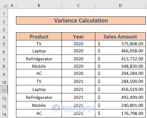
This is the dataset that I am going to use. We have some products and their sales amount.

calculate variance in excel pivot table

I will calculate the variance of sales amount for the years 2020 and 2021.


Step 1: Create a Pivot Table from Data Range

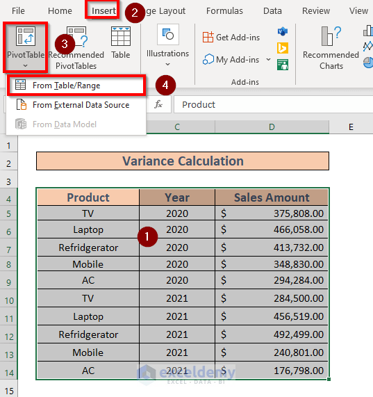
  • Select the range B4:D14. Then go to the Insert tab >> select Pivot Table >> select From Table/Range.

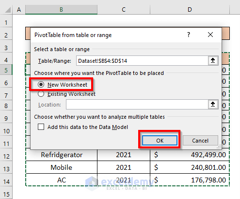
  • A new window will appear. Select New Worksheet to get a pivot table in a new worksheet. Then select OK.

calculate variance in excel pivot table

Excel will create a pivot table.


Step 2: Drag the Fields to Required Areas

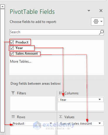
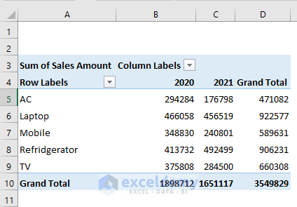
  • In the PivotTable Fields, put Product in the Rows, Year in the Columns, and Sales Amount in the Values

calculate variance in excel pivot tableThen the table will look like this.


Step 3: Remove Grand Total for Rows

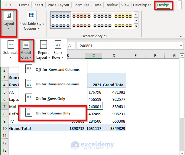
  • Now go to the Design tab >> select Layout >> select Grand Total >> choose On For Columns Only.
calculate variance in excel pivot table

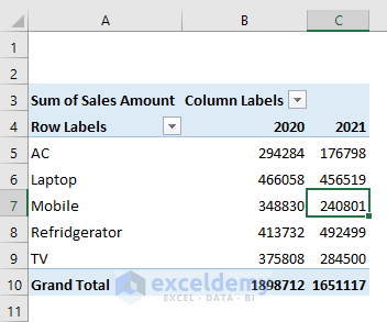
Excel will remove the Grand Total for Rows.

Step 4: Change Cell Format to Accounting

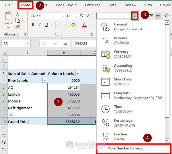
  • Now select the range B5:D10. Go to the Home tab >> select the drop-down (see image) >> select More Number Formats.

calculate variance in excel pivot table

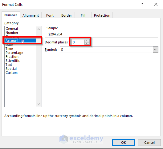
  • Format Cells box will appear. Select Accounting >> set Decimal Places as 0 >> Click OK.
Excel will change the format of the sales amounts.
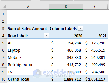
calculate variance in excel pivot table


Step 5: Calculate Variance as a Change in Percentage

  • Now put the Sales Amount to the Values field.

  • Now select the drop-down shown in the image >> select Value Field Settings.

calculate variance in excel pivot table

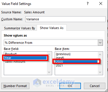
  • Now, the Value Field Settings window will pop up. Set the Custom Name Variance >> select Show Values as >> choose % Difference From.
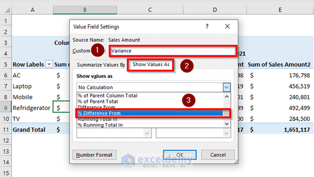
  • Now, select the Base field as Year and the Base item as 2020. Click OK.

calculate variance in excel pivot table

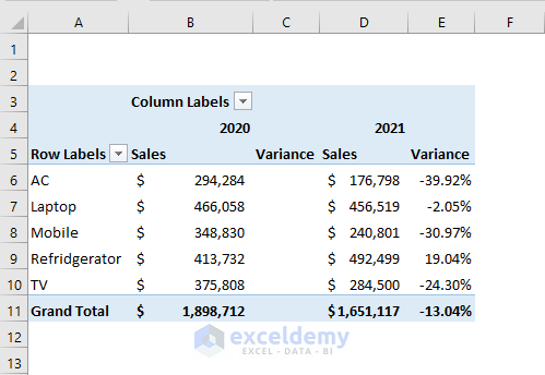
  • Excel will calculate the variance.

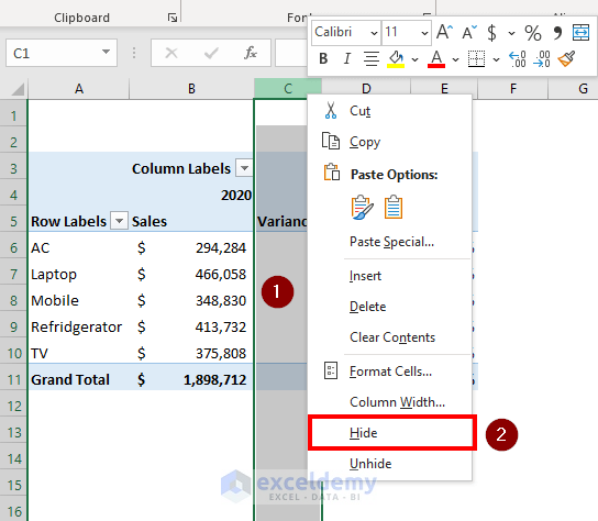
  • Now, select column C. Select Hide from the Context menu to hide the column.

calculate variance in excel pivot table

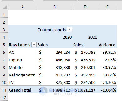
Your final output will be like this.


Things to Remember

  • This method is basically about calculating the variance in percentage between the sales data of two separate years. However, it is worth mentioning that this variance is different from statistical variance.

Download Practice Workbook

Download this workbook and practice while going through this article.


Conclusion

In this article, I have demonstrated an effective method to calculate variance in Excel Pivot Table. I hope it helps everyone. And lastly, if you have any kind of suggestions, ideas, or feedback please feel free to comment down below.


Related Articles


<< Go Back to Calculated Field in Pivot Table | Pivot Table Calculations | Pivot Table in Excel | Learn Excel

Get FREE Advanced Excel Exercises with Solutions!
Akib Bin Rashid
Akib Bin Rashid

AKIB BIN RASHID, a materials and metallurgical engineer, is passionate about delving into Excel and VBA programming. To him, programming is a valuable time-saving tool for managing data, files, and internet-related tasks. Proficient in MS Office, AutoCAD, Excel, and VBA, he goes beyond the fundamentals. Holding a B.Sc in Materials and Metallurgical Engineering from Bangladesh University of Engineering and Technology, MD AKIB has transitioned into a content development role. Specializing in creating technical content centred around Excel and... Read Full Bio

We will be happy to hear your thoughts

Leave a reply

Advanced Excel Exercises with Solutions PDF


ExcelDemy
Logo