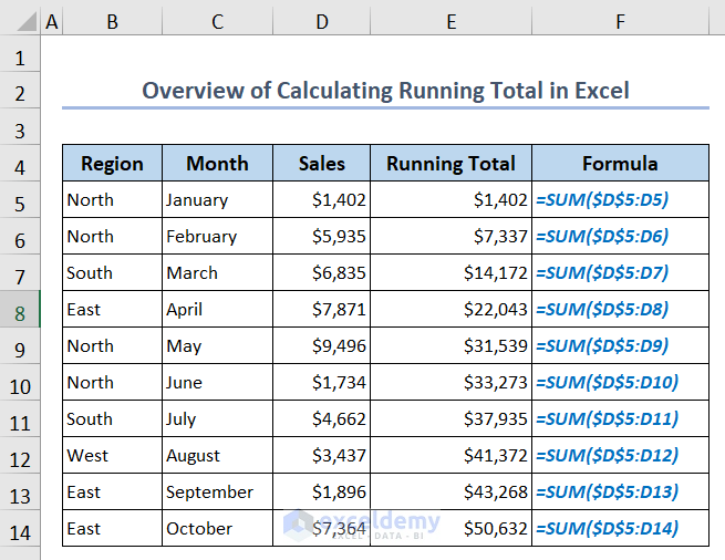
In the following overview image, we used the SUM function to calculate the running total of sales values, with the formulas showing how the function is updated through cells.
Download the Practice Workbook
What Is a Running Total?
A running total, or a cumulative sum, is a series of partial sums of any set of data. The running total shows the summary of data as it accumulates over time.
Suppose we have the first value X. If we get the second value Y, the running total will be X+Y. Similarly, if there’s a third value Z, the updated running total will be X+Y+Z, and so on.
What Are the Uses of Running Total?
- You can use it in the cash register operation of any store. Cash registers in particular show a running total of different products as they are scanned into the system. They usually keep track of all transactions that take place throughout the day in a running total as well.
- The running total is useful in sports. An excellent example of a running total is in the sport of cricket. Every time a player scores a run, the total run gets increased. As a result, the final score is only the aggregate of the runs or running total.
- You need to calculate the running total if you work in a sales position. If you have a quota, you can use a running total to monitor your progress. Managers use these running totals to assess the performance of workers on a monthly, quarterly, or annual basis.
- You can use the running total in the year-to-date calculation. The running total tracks a specific task or activity from a specific date until the end of the year.
- Businesses frequently use the running totals to manage their inventories as they have to keep track of how many goods are sold. Then, they compare that number to how many items they have on hand.
- You can use the running total in the balance sheet. You can clearly see any assets and liabilities at any time with the use of balance sheets.
- You can also use the running total for calculating your bank balance.
- Ride-sharing companies and delivery services use the running total to track the mileage. As a result, drivers are compensated per mile.
- You may track your daily or weekly calorie intake using the running totals. You can track your calories in order to lose weight. For this purpose, use Excel to input the number of calories in each meal. Then, calculate how many calories you’ll consume over the course of a day or a week.
How to Calculate the Running Total in Excel
Method 1 – Use a Custom Formula
- Use the following formula in cell E5 to get the first running total result.
=D5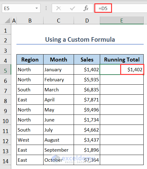
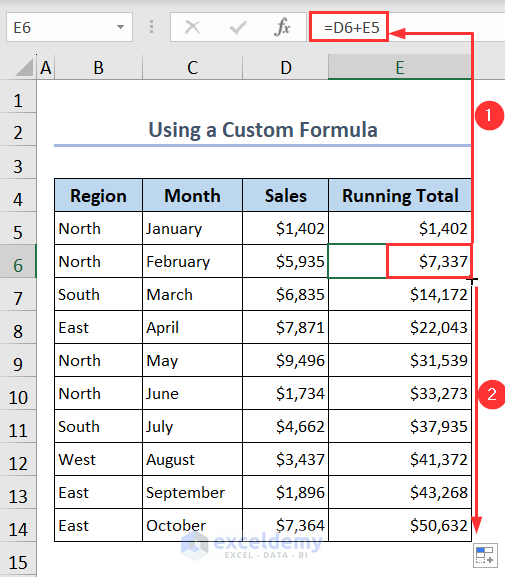
- Use the following formula in cell E6:
=D6+E5- Apply the Fill Handle tool to copy this formula in the rest of the column. You’ll get the running total.
Method 2 – Apply the SUM Function
- Insert the following formula in cell E5, then apply the Fill Handle tool to get the running total:
=SUM($D$5:D5)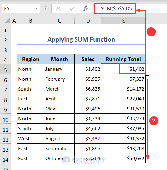
Method 3 – Use the SUMIF Function for Conditions
- Insert the following formula in cell E5, then apply the Fill Handle tool to get the running total for values that have “North” as the region.
=SUMIF($B$5:B5,"North",$D$5:D5)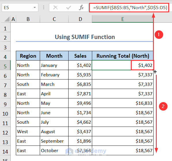
Method 4 – Combine SCAN and LAMBDA Function
- Insert the following formula in cell E5.
=SCAN(0,D5:D14,LAMBDA(a,v,a+v))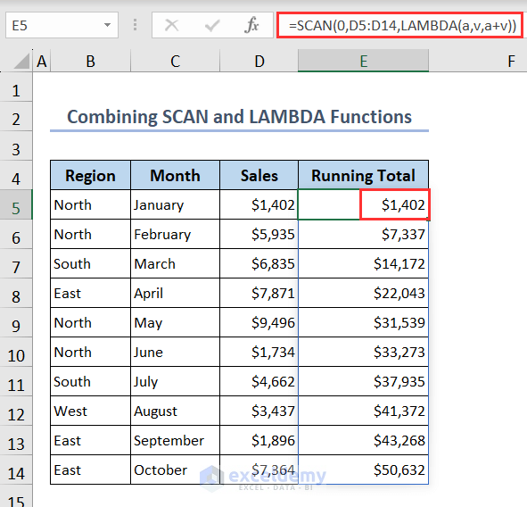
Formula Breakdown
- LAMBDA(a,v,a+v)– Here a represents the accumulated value and v represents the current value in the iteration. The expression a+v adds the current value to the accumulated value using the LAMBDA function.
- SCAN(0,D5:D14,LAMBDA(a,v,a+v))– Here the initial value is set to 0. Then, the second argument D5:D14 represents the range of values over which the SCAN function will iterate. Finally, the SCAN function performs the LAMBDA expression calculation for each value.
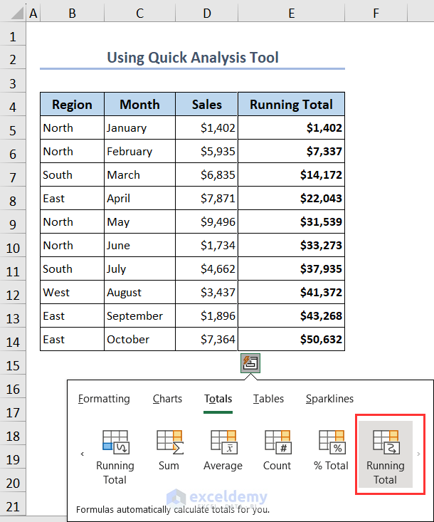
Method 5 – Use the Quick Analysis Tool to Calculate the Running Total Automatically
- Select the whole dataset and click on the Quick Analysis Tool button.
- Click on the Total tab and then press the slider button.
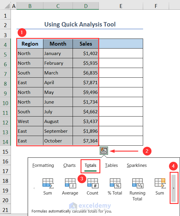
- Select Running Total (yellow color). You’ll get the running total of your values placed automatically in column E.
Method 6 – Use the Table Feature
- Select the whole dataset (B4:E14).
- Go to Insert and select Table. Or, press Ctrl + T from your keyboard.
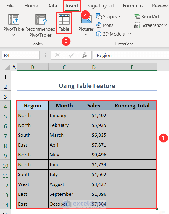
- Tick the option My table has headers in the Create Table window.
- Press OK.
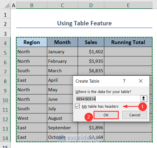
- The Table is ready to use.
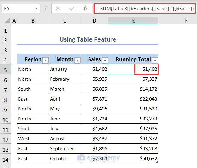
- Put the following formula in cell E5:
=SUM(Table3[[#Headers],[Sales]]:[@Sales])We use Table3 as our table’s name and we summed the Sales column of our table.
Method 7 – Apply Power Query
- Select the whole dataset.
- Go to Data and choose From Table/Range.
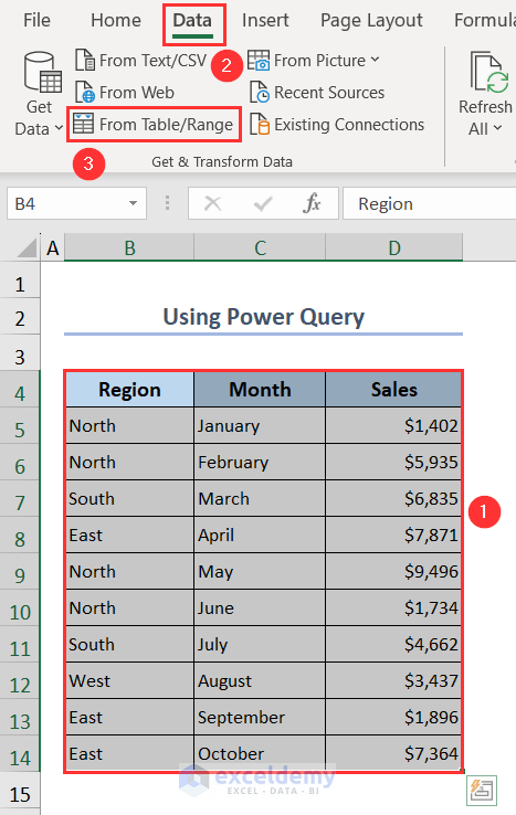
- In the Create Table window, tick the option My table has headers.
- Press OK.
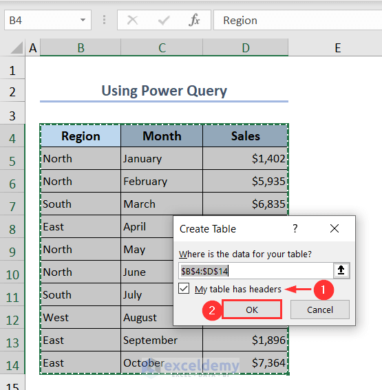
The Power Query Editor will open.
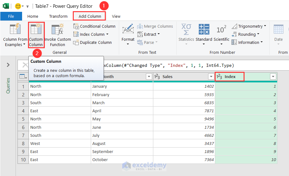
- Go to the Add Column tab and select From 1 from the Index Column drop-down menu.

- A new column titled Index will be added next to the Sales column.
- Select Custom Column under the Add Column tab.
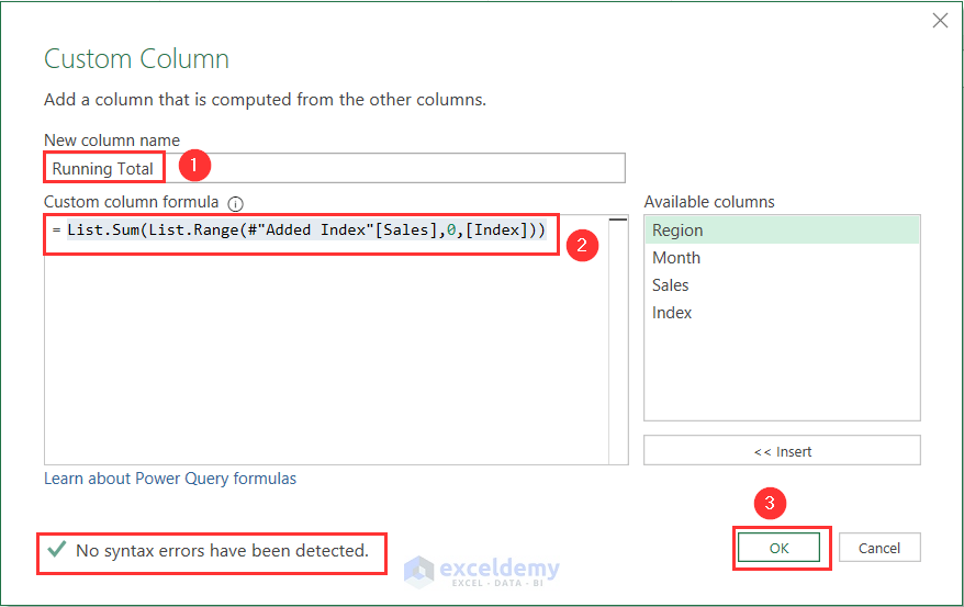
- In the Custom Column window, type a new column name. We put Running Total as the name.
- Put the following formula in the formula box:
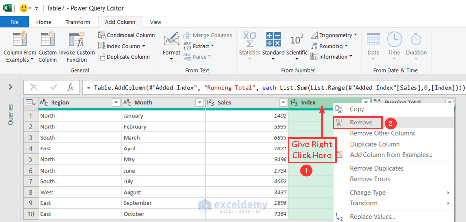
=List.Sum(List.Range(#"Added Index"[Sales],0,[Index]))Sum gives the sum of the range within the dataset. List.Range gives the range of Sales and it will change depending on the Index value.
- Check whether No syntax errors have been detected appears. If it appears, press the OK button. If you get an error, re-check the formula.
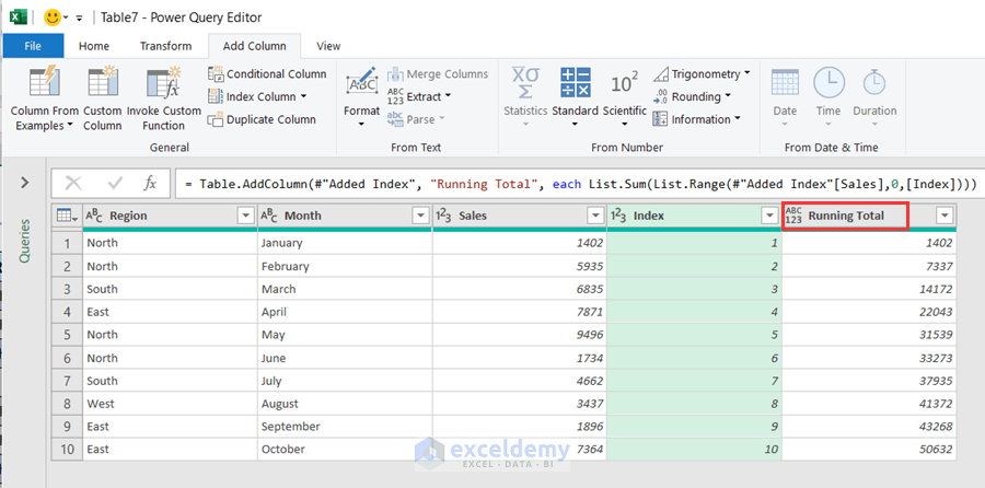
- A new column titled Running Total will be added after the Index column.
- Right-click on the empty space of the Index column.
- Select the Remove option.
- Go to the Home tab and select Close & Load.

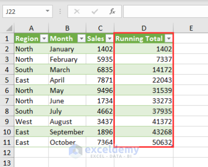
You’ll get the running total of your sales values along with the dataset in a new worksheet.
Method 8 – Use a Pivot Table
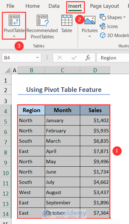
- Select B4:D14 and go to Insert, then choose PivotTable.
- Choose the option New Worksheet in the PivotTable from table or range window.
- Press OK.

- The PivotTable Fields window will open.
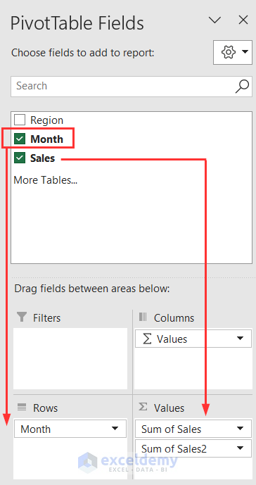
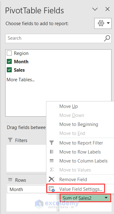
- Drag the Month under the Rows field once and the Sales under the Values field twice.
- You’ll get a dataset like below.
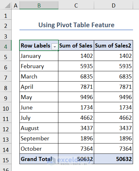
- In the PivotTable Fields window, go to the Value Field Settings by clicking on the Sum of Sales2 drop-down.
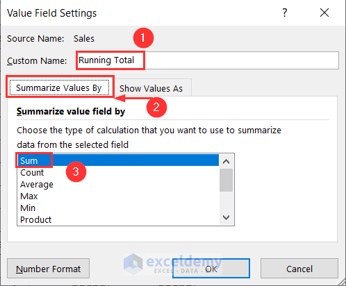
- In the Value Field Settings wizard, put the name as Running Total.
- Go to Summarize Values By tab and choose Sum from the drop-down.
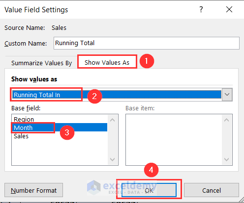
- Go to the Show Values As tab and choose Running Total In under this option.
- Select Month as the Base field and press OK.
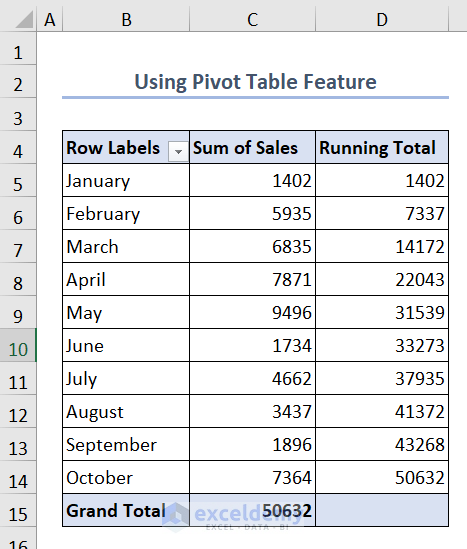
- You’ll see the running total in column D.
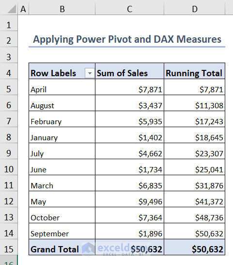
Method 9 – Apply Power Pivot and DAX
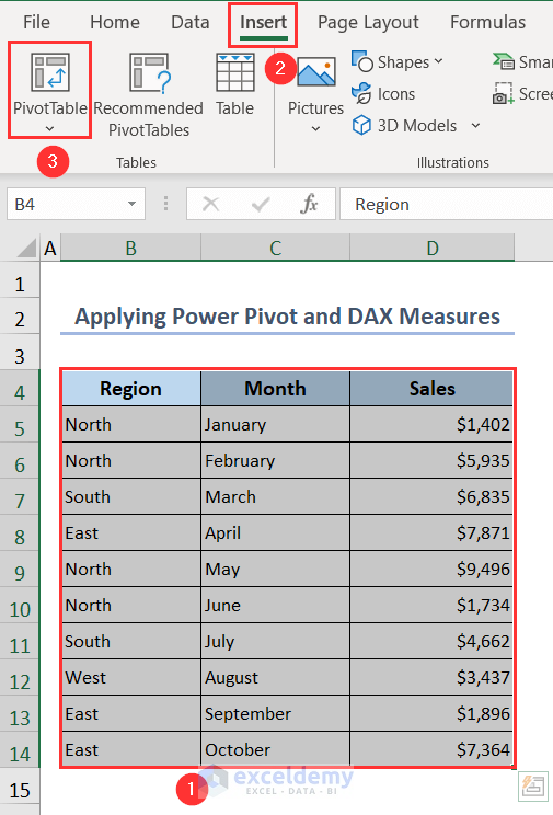
- Select B4:D14, go to Insert, and choose PivotTable.
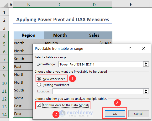
- Choose New Worksheet and tick the option Add this data to the Data Model in the PivotTable from table or range window.
- Press OK.
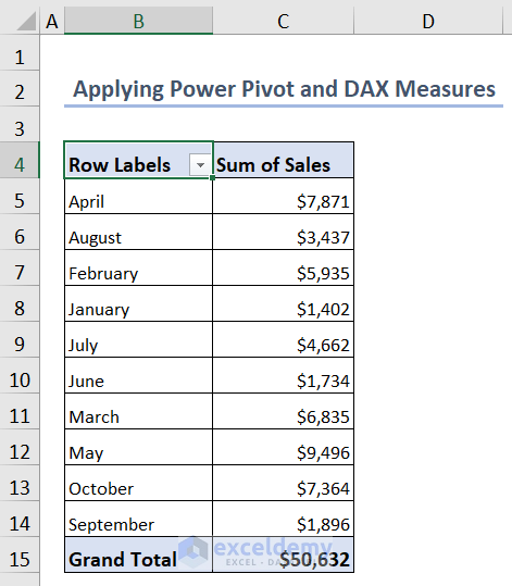
- Select Month and Sales. These 2 will automatically get added to the Rows and Values fields, respectively, under the PivotTable Fields pane.
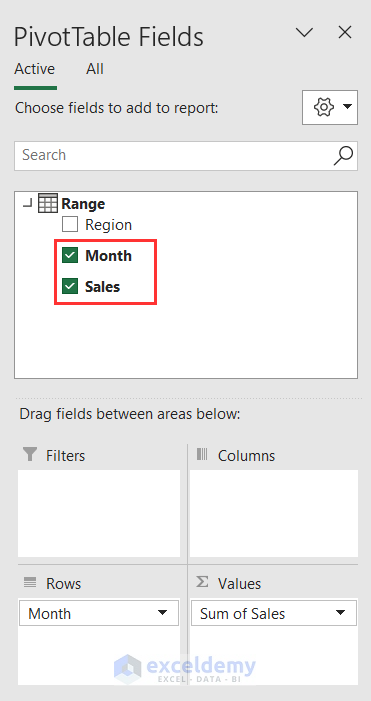
- You’ll see a dataset like this in your Excel sheet.
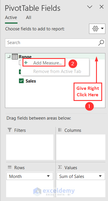
- In the PivotTable Fields pane, right-click on the empty space of Range.
- Click on the Add Measure option.
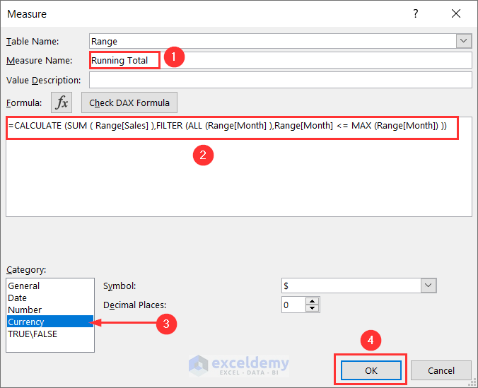
- You’ll get the Measure window. Give it a name like Running Total.
- Put the DAX formula in the formula box:
=CALCULATE (SUM ( Range[Sales] ),FILTER (ALL (Range[Month] ),Range[Month] <= MAX (Range[Month]) ))Range[Sales] refers to the Sales column and Range[Month] indicates the Month column of the dataset.
- Select Currency as the Category and press OK.
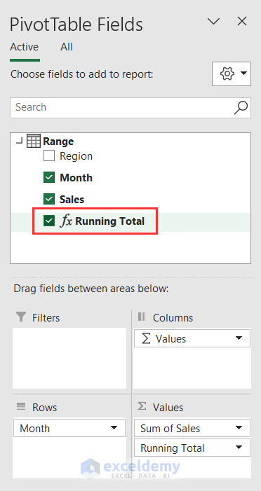
- Running Total is added in the PivotTable Fields window.
- Tick it to add this to your Excel sheet.
You’ll obtain the running total of the sales values.
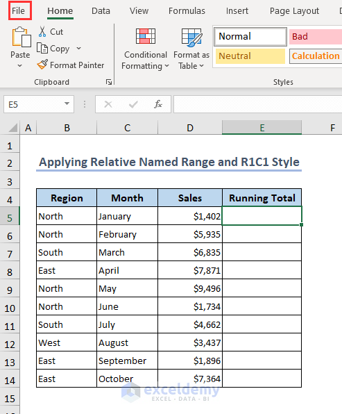
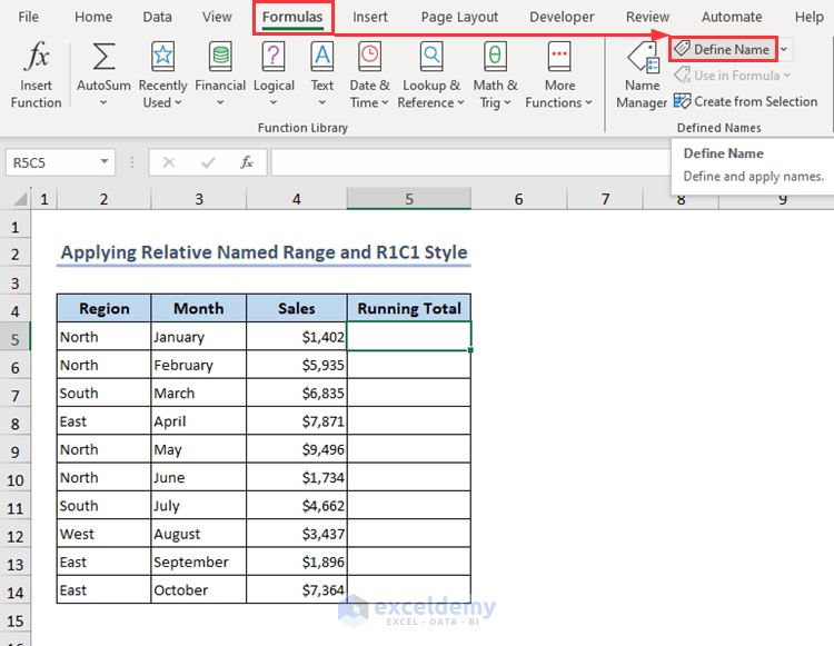
Method 10 – Apply a Relative Named Range and R1C1 Style with the SUM Function
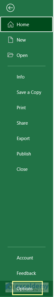
- Go to the File tab.
- Select Options under the Home tab.
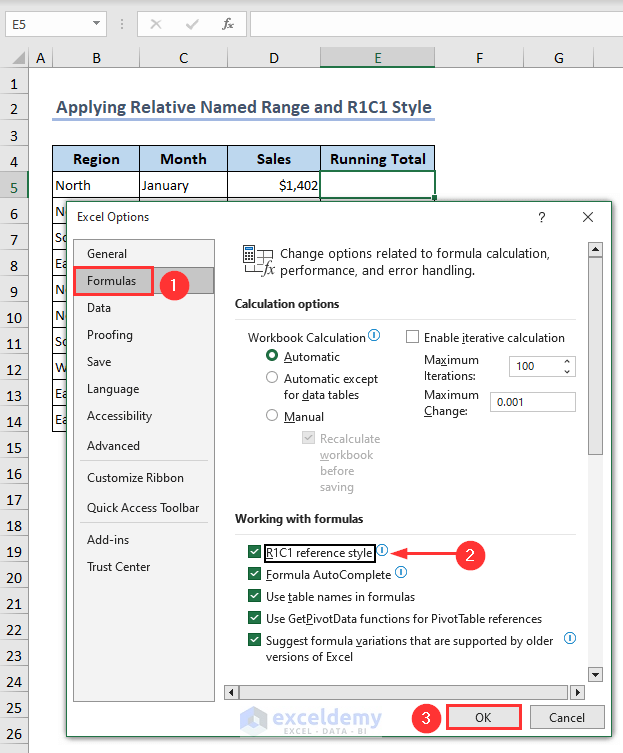
- The Excel Options window will open up.
- Tick the R1C1 reference style option from the Formulas tab.
- Click OK.
- The reference style will change to R1C1 (shown by column letters being replaced with numbers).
- Go to Formulas and choose Define Name.
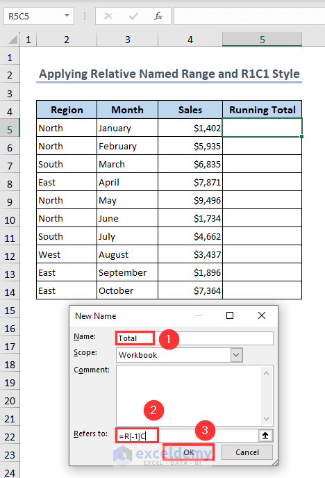
- The New Name window will open up.
- Put a name Total in the Name box.
- Insert the following formula in the Refers to box.
=R[-1]C- Click OK.
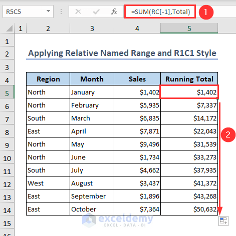
- Put the following formula in cell R5C5 and apply the Fill Handle tool:
=SUM(RC[-1],Total)You’ll obtain the running total of the sales values.
How to Create a Running Total Chart in Excel
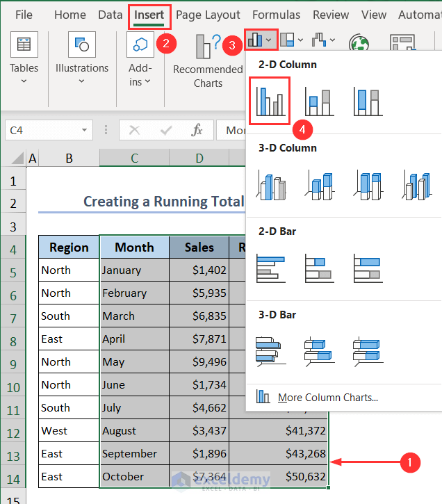
- Select the whole dataset excluding the Region column (C4:E14).
- Go to the Insert tab.
- Select 2D Clustered Column Chart from the Column Chart options.
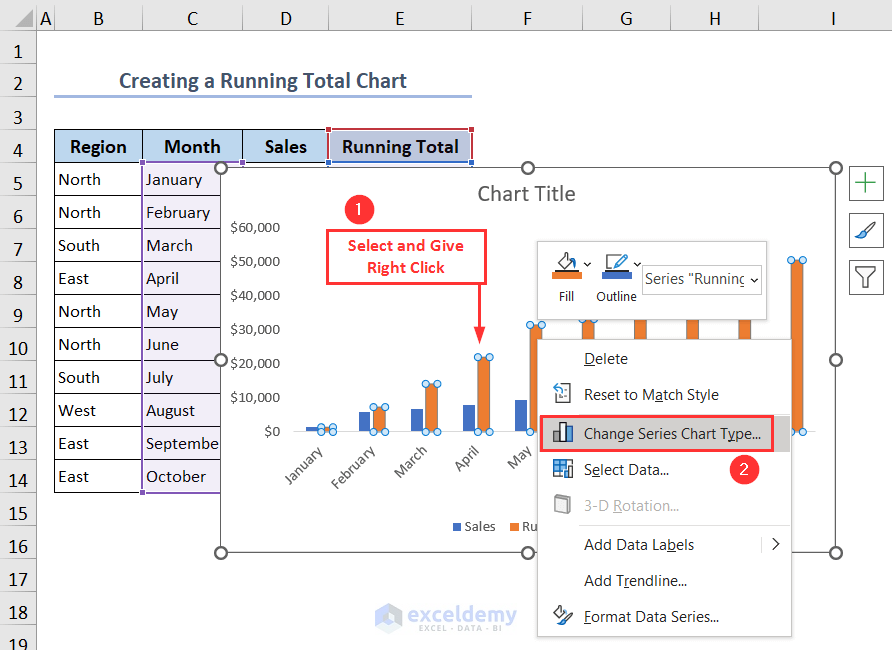
- Select the Running Total Columns (Orange Color) and right-click.
- Select Change Series Chart Type.
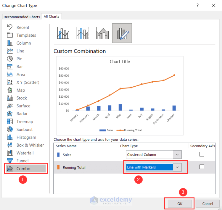
- Go to the Combo tab in the Change Chart Type window.
- Select Line with Markers for Running Total Chart and press OK.
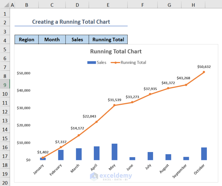
- The chart is now ready.
- We have made some formatting changes like giving the chart a title and adding a legend to make the chart visually appealing.
Things to Remember
- A running total and the total sum are different. The running total sums the former value with the current value. But the total sum sums all the values.
- The running total is different from the running balance. In the running balance, when you add a new entry, the sum of values can grow or reduce. But in the running total, it’ll only grow.
- When we used the Named Range method, we changed the reference style to R1C1 from A1 style. This change is only applicable to this method.
Frequently Asked Questions
What is an example of a running total?
Suppose you work in a sales position and want to know the total number of items sold up to a particular date. In this case, you have to calculate the running total of the number of items sold instead of the sum.
What is the formula for a running balance in Excel?
There are a lot of formulas for a running balance in Excel. You can use a custom formula and SUM, SUMIF, SCAN, and LAMBDA functions to calculate the running balance. You’ll find all these methods in this article.
What is the purpose of running total in Excel?
The purpose of the running total in Excel is to add up the values of items as we enter new items and values over time.
What are the methods available to find the running total in Excel?
In this article, you’ll find all the methods available to find the running total in Excel. We can apply a custom formula and use SUM, SUMIF, SCAN, and LAMBDA functions to calculate the running total. Moreover, we use the Quick Analysis tool, Table, Pivot Table, Power Query, Power Pivot, and DAX measures.
Excel Running Total: Knowledge Hub
<< Go Back to How to Calculate in Excel | Learn Excel
Get FREE Advanced Excel Exercises with Solutions!
