The cost of funds is the interest rate that banks and financial institutions pay on the money they utilize for their operations. Generally, this cost can be calculated manually. You can determine the cost of funds by using the following formula.
LTP = Long Term Debt Proportion.
PSP = Proportion of Preferred Stock and.
CSP = Proportion for Common Stock.
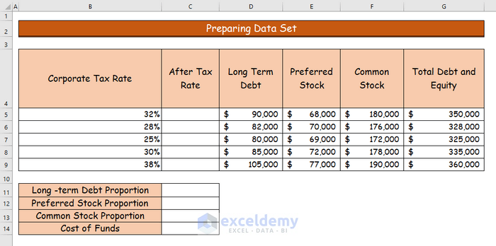
Step 1 – Preparing the Data Set
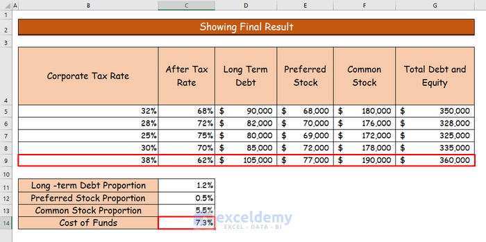
- Insert the following data set. We will input values for Corporate Tax Rate, Long Term Debt, Preferred Stock, Common Stock, and Total Debt and Equity.
Step 2 – Determining the After-Tax Rate
- Apply the following formula in cell C6 to find out the after-tax rate for the corporate tax rate of 32%.
=1-B5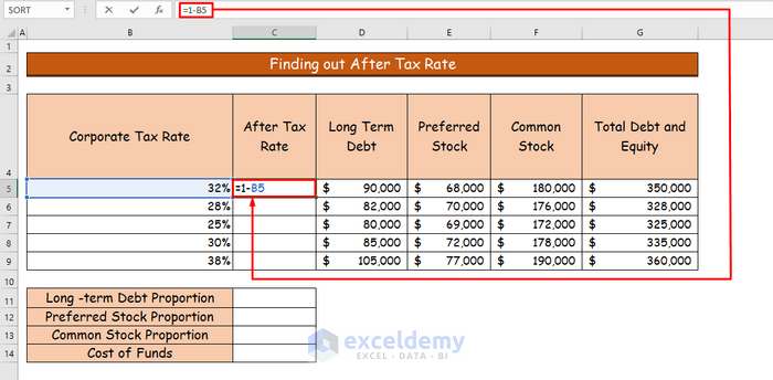
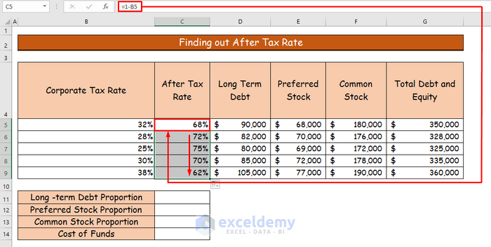
- Hit Enter to get the value of the after-tax rate.
- Use AutoFill to get the after-tax rate for the other cells.
Step 3 – Calculating the Proportion for a Long-Term Debt
In our example, the long-term debt for the first case is $90,000 with an unchanged interest rate of 7%.
- Use the following formula in the formula bar for cell C11.
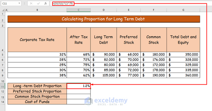
=(D5/G5)*C5*7%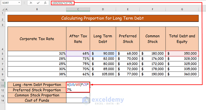
- Here’s the result.
Step 4 – Determining the Proportion of Preferred Stock
In our sample, the preferred stock for the first case is $68,000 with a percentage rate of 2.5%.
- Use the following formula in cell C12 to determine the proportion of preferred stock.
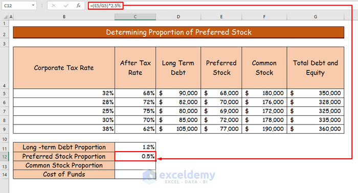
=(E5/G5)*2.5%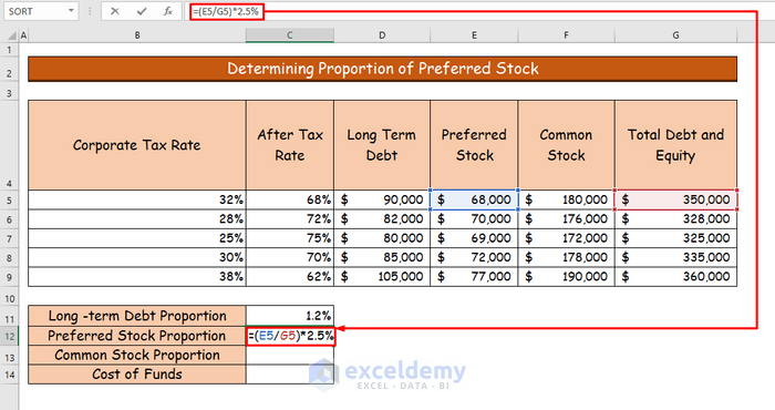
- Hit Enter.
Step 5 – Determining the Proportion of Common Stock
For our dataset, the amount of common stock is $180,000 with a minimum amount of profit return of 12%.
- In cell C13, use the following formula.
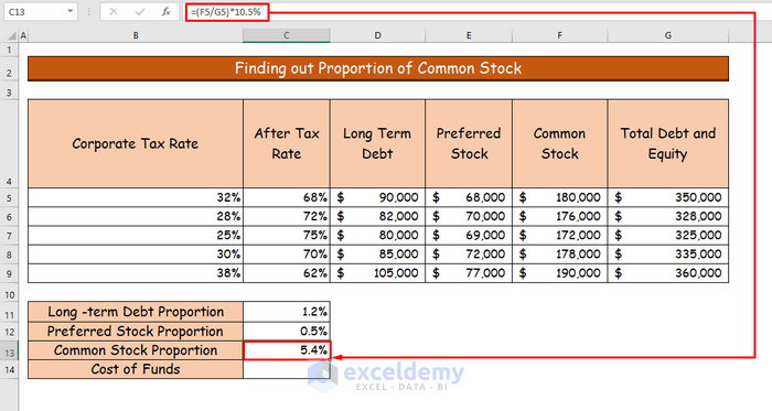
=(F5/G5)*10.5%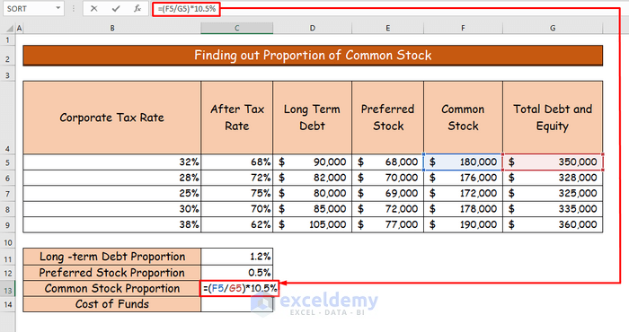
- Hit Enter.
Step 6 – Adding up All Proportions to Calculate the Cost of Funds
- Use this formula in cell C14.
=SUM(C11:C13)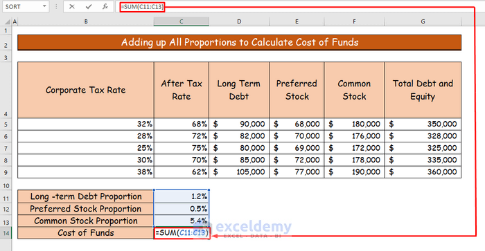
- Hit Enter.
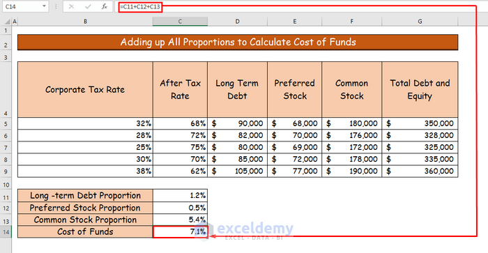
Step 7 – Showing the Final Result
Importance of Cost of Funds
- If the cost of funds is higher, the financial institution will impose more interest on loan borrowers to compensate for the cost.
- If the cost of funds is lower, the institutions can give loans at a lower interest rate.
- The loan borrower has to pay less interest on their loan if the cost of funds is minimized.
Download the Practice Workbook
<< Go Back to Cost | Formula List | Learn Excel
Get FREE Advanced Excel Exercises with Solutions!
