Method 1 – Calculate the Area under a Scatter Plot in an Excel Sheet
1.1 Using Trapezoidal Rule
Steps:
- Insert a scatter plot for the dataset. Select the dataset >> go to the Insert tab >> click the Insert Scatter or Bubble Chart tool >> select the Scatter with Smooth Lines option.
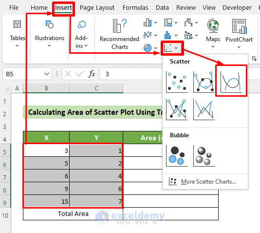
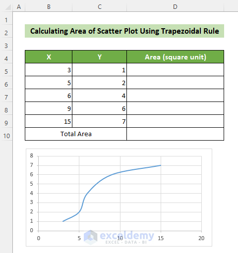
- See that the dataset has a scatter plot now.
- Select the D5 cell and insert the following formula.
=(C5+C6)/2*(B6-B5)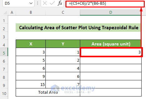
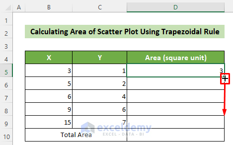
- Get the enclosed area between the 5th and 6th-row datasets. Place the cursor in the bottom right position of the D5 cell.
- The fill handle will appear. Drag the fill handle downward to copy the formula to all the cells up to row 8.
Note:
The formula isn’t copied to row 9, because it is the last point of the plot. It does not enclose any mentionable area.
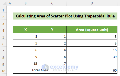
- The D10 cell, write the following formula to sum all the enclosed areas individually between two intervals.
=SUM(D5:D9)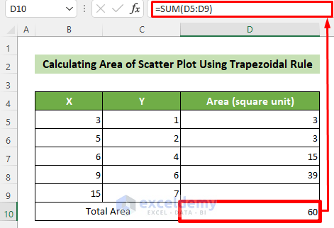
Note:
The SUM function is a function that is used to sum multiple numbers. It has the arguments which require the numbers that you want to sum up.
Find the total area enclosed by the scatter plot using this method. The overall result sheet will look like this.
1.2 Using Excel Chart Trendline and Mathematical Integration
Steps:
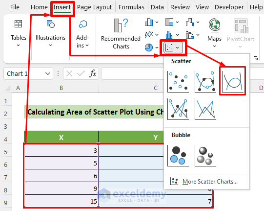
- Select the required columns of your dataset, which are column B and column C.
- Go to the Insert tab >> click the Insert Scatter or Bubble Chart tool >> select the Scatter with Smooth Lines option.
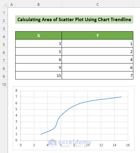
- Get the scatter plot of your dataset.
- Cick on the Chart Elements icon >> click the rightward arrow beside the Trendline option >> choose the More Options… option from the context menu.
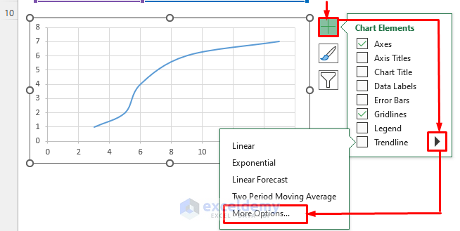
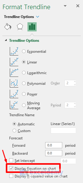
- A new ribbon named Format Trendline will appear on the right side. Put the tick mark on the Display Equation on chart option.
- See a trendline will appear along with the equation on your chart.
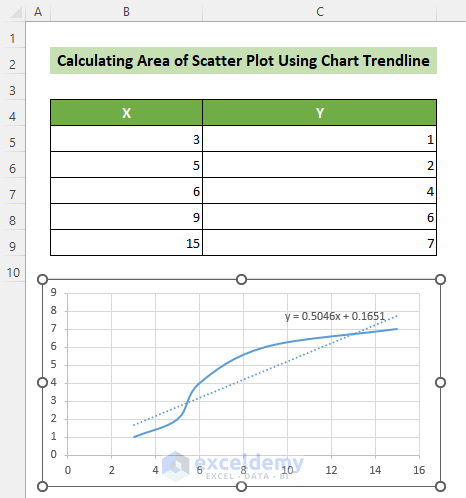
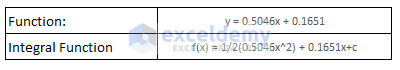
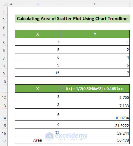
- Calculate the area, you need to find the integral function of the equation. For better visualization, write the trendline equation and integral function.
- Build a new table for the value and the integral value of the function concerning x.
- Click on the C16 cell and write the following formula which we have got earlier by integrating the trendline equation.
=1/2*(0.5046*B16^2)+(0.1651*B16)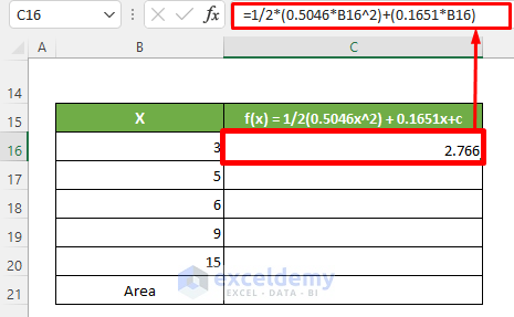
- You will get f(3) by applying this formula. Because you have used 3 as x’s value.
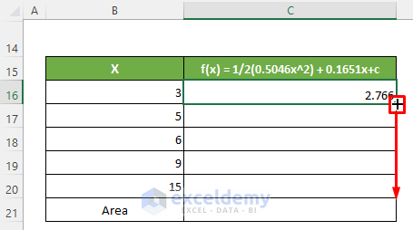
- Put your cursor in the bottom right position of the cell. You will see the fill handle will appear. Drag the fill handle downward to get all the other f(x) for all the x’s values.
- The last x’s f(x) and the first x’s f(x). Calculating the area, click on the C21 cell and write the following formula.
=C20-C16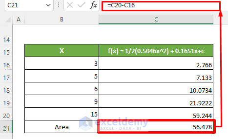
Get the area enclosed by the scatter plot successfully by doing this. The result sheet should look like this after the result.
Method 2 – Calculate the Area of Different Geometric Shapes
Steps:
- Click on the D5 cell where you want to calculate your triangle area. Write the formula below on the cell.
=0.5*B5*C5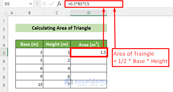
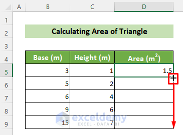
- Get the area of the first triangle. Place your cursor in the bottom-right position of the D5 cell.
- Fill handle will appear. Drag the fill handle below to copy the area formula for all the cells below.
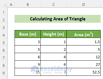
Find the area of all triangles. The result sheet will look like this.
2.2 Area of Rectangle
Steps:
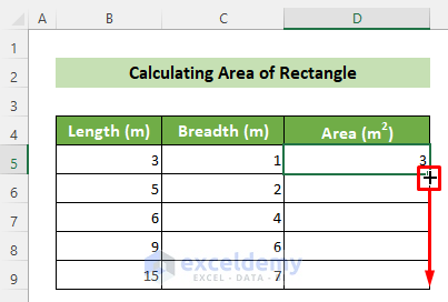
- Click the D5 cell where you want to put your result. Insert the following formula in the D5 cell.
=B5*C5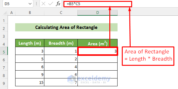
- Get the area of the first rectangle. Place your cursor in the bottom right position of the selected cell.
- The fill handle will appear. Drag the fill handle below to all the cells.
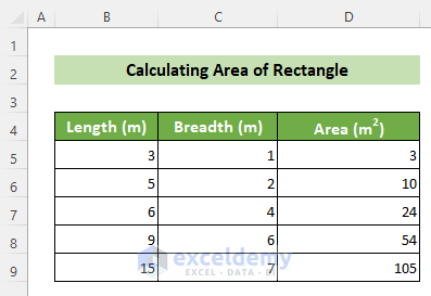
Calculate all the rectangle’s areas. The result sheet should look like this.
2.3 Area of Square
Steps:
- Click on the C5 cell and write the following formula.
=POWER(B5,2)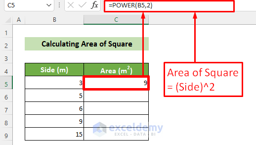
Note:
The POWER function is the function that is used to calculate the definite power of a definite number. It has two arguments, such as number and power. The number argument takes the number that needs to be powered. The power argument takes the digit to which the following number should be powered.
- Get the area of a square. Place your cursor on the bottom right of your selected cell, and upon the appearance of the fill handle, drag it downward.
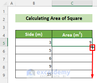
- The formula will be copied to all the cells.
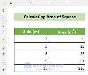
Get all the squares’ area, the result sheet would look like this.
2.4 Area of Circle
Steps:
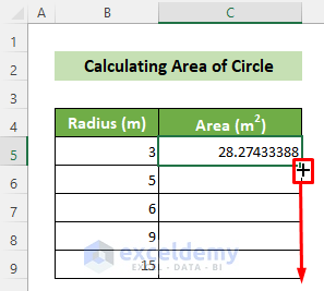
- Click on the C5 cell as you want your result in this cell. Write the following formula in the cell.
=PI()*POWER(B5,2)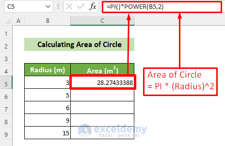
- Find the area of the first circle of your dataset. Place your cursor in the bottom right position of your cell.
- The fill handle will appear. Drag the fill handle downward to copy the area formula for all the cells below.
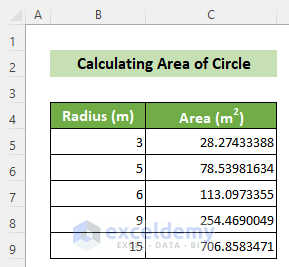
Calculate the area of squares in the Excel sheet. You can see the result like this.
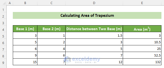
2.5 Area of Trapezium
Steps:
- Click on the E5 cell where you want to calculate the area of the trapezium. Put an equal sign (=) to start the formula. Insert the following formula in the cell.
=((B5+C5)/2)*D5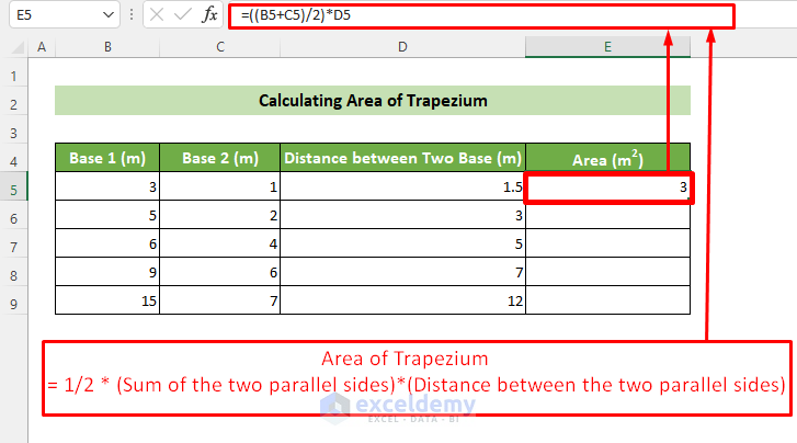
- Get the area of the first trapezium of your dataset. Place your cursor in the bottom right position of the E5 cell.
- The fill handle will appear. Last but not least, drag this fill handle downward to copy the trapezium area formula for all the other given dimensions of the trapezium.
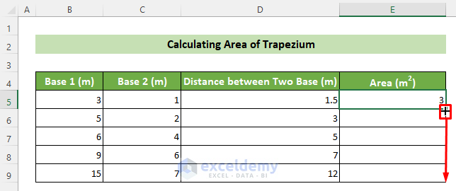
Find all the areas of all the trapeziums. For example, the result sheet will look like this.
Download Practice Workbook
You can download and practice from our workbook here for free.
<< Go Back to Formula List | Learn Excel
Get FREE Advanced Excel Exercises with Solutions!
