Latest Posts From Shajratul Alam Towhid

We need to calculate the average price in various business sectors or normal life frequently. Excel has made it easy to calculate the average price. There are ...

We have made a dataset of Sales of Shoes and Bags in 2021 at different stores. We'll use it to apply various range functions. Method 1 - Applying ...

There are thousands of cells in an Excel sheet. Every time we need to edit those cells because there is data, values, formulas, and so on in a cell and we need ...
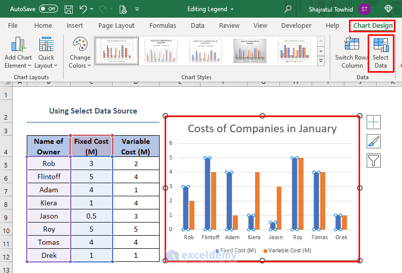
While using charts in Excel we often need to edit the legend. Legends are basically representation of data. We mainly use legends when data has the same type ...

Converting one dimension to another dimension seems to be a difficult task most of the time. We need to convert inches to mm, mm to feet, kg to pound, and so ...

Dataset Overview To convert inches to mm in Excel, we have made a dataset of the vertical Distance (in Inch) of pumps from the basement of an effluent ...

We have made a sample dataset for some companies. We will use the Fill Handle tool both vertically and horizontally. Example 1 - Copying a Formula ...

Here is an overview of how to insert a scroll bar in the Excel worksheet using the Developer tab. 2 Ways to Insert Scroll Bar in Excel There are ...
- « Previous Page
- 1
- …
- 3
- 4
- 5
See Our Reviews at


Dear Nelly,
Actually, percentage change mostly fits between two numbers. There is no specific formula to calculate percentage change among multiple numbers. Rather, when we face percentage change calculation, it means we are simply asked for the percentage change between the first number and the last number. In this case, the formula is.
=((Final Value – Initial Value)/Initial Value)*100
As your teacher has given you 10 different columns of values, you can calculate percentage change for each 2 individual columns and finally find a mean value of percentage change.
This is like.
=((2nd Value – First Value)/First Value)*100
Then,
=((3rd Value – 2nd Value)/2nd Value)*100
Similarly, following the same formula find all the individual percentage change. For 10 columns you will find 9 individual percentage change.
Finally, to find the mean.
=(Percentage Change of (Step 1 + Step 2 + …….+ Step 9))/ 9
Similarly, this statement is true for calculating count.
Regards,
Towhid
Excel & VBA Content Developer
ExcelDemy
Dear Gen,
You can use the formula.
=TEXTJOIN(delimiter,TRUE,cell_range)
Here, for E5 cell you can write.
=TEXTJOIN(“-“,TRUE,B5:D5)
Here, the character “-” is used to separate the combined text.
This TEXTJOIN function is available only in Office 2019 and Microsoft 365.
The Excel TEXTJOIN function joins multiple values from a row, column or range of cells with specific delimiter.
For other versions of Excel, you can write the formula in the E5 cell based on B5,C5 and D5 cells like.
=B5&IF(C5<>“”,”-“&C5,””)&IF(D5<>“”,”-“&D5,””)
Finally, you need to set your column width to place the output in the cell perfectly and also need to wrap text.
By using either of these two formulas you can ignore empty cells to combine cells into one.
Regards,
Towhid
Excel & VBA Content Developer
ExcelDemy
Dear William Moloney,
As far as I understand, you are able to use “Format Cell” but can’t get the procedure of using “Control Panel” to fix negative number format, right?
You are using Windows 10 and you can do it easily in Windows 10.
Firstly, go to “Control Panel”.
Secondly, click on “Change date, time and number format” in the option “Clock and Region”.
Thirdly, a window named “Region” will appear. Go to “Formats” option of that window. Click on “Additional settings” at the right-bottom side of the window.
You will see a “Customize Format” window. Go to “Numbers” of this window. You’ll see many options available in this “Numbers” option.
Fourthly, in the “Negative Number Format” option, click on the value and you will see different options such as 1.1, -1.1, 1.1- etc. You need to select 1.1 here and then click OK. This is the most important step here to select 1.1. Windows 10 has default selection 0f -1.1, you need to just change it to 1.1.
Hope, your problem will be solved now. Thank you.
Regards,
Towhid
Excel & VBA Content Expert
ExcelDemy
Hello RAY,
Can you please elaborate what problems you are facing? And the problems in getting the output using these methods? I mean, the output scenario needs to be known and analyze properly to make a solution of your problem.
Thanks with Regards,
Towhid
Excel and VBA Content Developer
Hello NK,
It’s awesome that you have found another solution which is applicable by adding a simple symbol in the formula you have mentioned. Yes obviously it is possible to remove blank from lists using the combination of UNIQUE and FILTER functions. The formula should be for the dataset of this article.
=UNIQUE(FILTER(B5:B14,B5:B14<>“”))
You need to add the symbol <> extra.
Here, the FILTER function is used to remove any blank values from the data.
The <> symbol is a logical operator that means does not equal.
The filtered data is returned directly to the UNIQUE function as the array argument. The UNIQUE function then removes duplicates and return the final array.
Thanks with Regards,
Towhid
Excel & VBA Content Developer