Md. Aniruddah Alam, a graduate of Bangladesh University of Engineering & Technology, Dhaka, holds a BSc.Engg in Naval Architecture & Marine Engineering. Joining Softeko in August 2022 as an Excel and VBA content developer, he has authored 90+ articles, covering fundamental to advanced Excel topics. He actively develops VBA codes for Excel automation and offers solutions in the Exceldemy Forum. Beyond work, he finds leisure in reading books, and taking relaxing walks, showcasing well-rounded blend of professional and personal interests.
Designation
Excel & VBA Content Developer at ExcelDemy in SOFTEKO.
The dataset showcases phone numbers before and after changing their formatting.
Changing Inconsistently Formatted Phone Numbers to a Specific Format ...
Thank you for sharing your problem. You may be experiencing the same issue as MICHAEL who shared his problem in the comment section above. Please try the solution suggested by Yousuf and let us know if the problem still persists. You can also share your file in our forum for us to investigate the issue closely.
Best of luck.
Thanks for reaching out to us! Unfortunately, the method discussed above doesn’t currently support recording half-day leave. We understand how frustrating that can be, and we’re sorry for any inconvenience caused. Rest assured, we’ll definitely work on overcoming this limitation in the future.
We’re grateful for your support of Exceldemy and we hope to make your experience even better in the future.
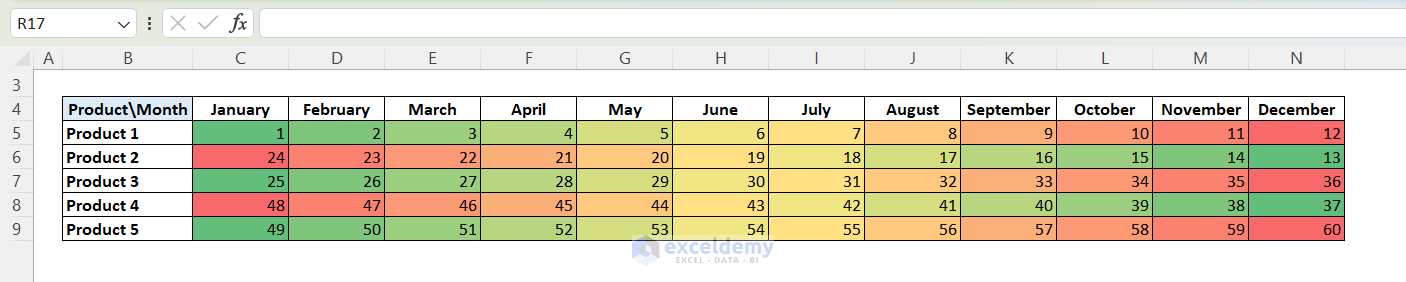
Thank you for sharing your problem with us. Yes, you are right that when you apply the conditional formatting (color scale) to the entire range,it ranks by each column, not by each row. Hence, in this case, to rank them by rows, you need to apply the conditional formatting to all the rows one by one. I have created a dataset based on your information and applied the conditional formatting to all the rows separately and got the expected result.
If you need to do this kind of stuff frequently, using VBA is indeed the best option as you mentioned.
Regards
Aniruddah
Team Exceldemy
Thanks for reaching out! Could you please explain a bit more about what you want to do? I wasn’t able to fully understand your comment. Do you need to get all the permutations? Let us know in the reply.
Dear Mary,
You can use the following code that also includes signature.
Sub ExcelToOutlookSR()
Dim mApp As Object
Dim mMail As Object
Dim SendToMail As String
Dim MailSubject As String
Dim mMailBody As String
Dim Signature As String
' Your signature text goes here
Signature = "Best regards," & vbCrLf & "Mary Rose"
For Each r In Selection
SendToMail = Range("C" & r.Row)
MailSubject = Range("F" & r.Row)
mMailBody = Range("G" & r.Row) & vbCrLf & vbCrLf & Signature ' Add the signature
Set mApp = CreateObject("Outlook.Application")
Set mMail = mApp.CreateItem(0)
With mMail
.To = SendToMail
.Subject = MailSubject
.Body = mMailBody
.Display ' You can use .Send
End With
Next r
End Sub
Dear DANIELLA,
Thanks for your comment. Have you tried the methods mentioned in this article to solve the issue? If you need further assistance, you can share your file in our Exceldemy Forum (https://exceldemy.com/forum/).
Dear Perry,
Thanks for your comment. Unfortunately, Excel does not have a Military time format. However, we can use the custom format feature in Excel to display military time. Follow the steps below to do so:
First, store the military time in text format. I store them as text format in cell C3 and C4 by selecting the cells and selecting “Text” from the Number group on Home tab.
Then, to add the times, use the following formula in cell B4: =TEXT((TIME(LEFT(C2,2),RIGHT(C2,2),0)+TIME(LEFT(C3,2),RIGHT(C3,2),0)),”hhmm”)
Formula Breakdown:
LEFT(C2,2) and RIGHT(C2,2): Extract the hours and minutes from cell C2.
LEFT(C3,2) and RIGHT(C3,2): Extract the hours and minutes from cell C3.
TIME(…): Create time values for the extracted hours and minutes.
TIME(LEFT(C2,2),RIGHT(C2,2),0)+TIME(LEFT(C3,2),RIGHT(C3,2),0): Add the times
TEXT(…, “hhmm”): Format the time difference as Military Times.
Note: Ensure that cells C2 and C3 are formatted as text to prevent Excel from automatically converting the time values. If Excel interprets them as time values, it may not work as expected. Also, if the total time exceeds 24 hours, it will not return the correct result. To address the issue, we have to create a custom function that requires VBA coding. If this solution does not meet your requirements, you can ask for a a customized solution on our Exceldemy Service.
Thank you for raising a valid concern about preserving text data in Excel. I completely agree that the current limitation, preserving only the upper-left value during a merge, can be frustrating.
To address this, I suggest exploring the five methods mentioned earlier to find the most suitable workaround for your specific case. Additionally, let’s hope that Microsoft Excel considers implementing a new merge option in the future, one that preserves all cell data.
Your feedback is valuable, and we appreciate your engagement.
Thanks for reaching out to us. Unfortunately, Conditional Formatting cannot create a vertical progress bar. But, using Sparkline can help you achieve your goal. You mentioned using Sparkline, but we didn’t understand what you meant by “not the entire range is filled.” Could you please clarify that?
Here’s a sample picture of a vertical progress bar that we created using Sparkline.
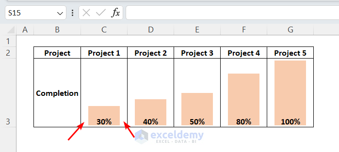
Were you referring to the extra space on the two sides of the column, as marked in the picture? If so, we are currently unaware of any methods to eliminate the space. Please let us know your thoughts.
Dear Amedeo,
Perhaps you are trying to break the file level protection. Unfortunately, the Zip method can only break the password on worksheet level or workbook level protection. Although this information may not have been highlighted earlier, is now included in a Note.
Regards
Aniruddah
Team Exceldemy
Thanks Nicu for reaching us out. To delete odd or even numbers in a range, you can use the following VBA Code:
Sub DeleteEvenOdd()
Dim Typ As String
Dim Rng As Range
On Error Resume Next ' Ignore errors if the user cancels the range selection
Set Rng = Application.InputBox("Select a range to delete Numbers", Type:=8)
On Error GoTo 0 ' Reset error handling
If Rng Is Nothing Then
Exit Sub ' User canceled range selection
End If
Typ = Application.InputBox("Put 1 for deleting Odd Number or 0 for Even Number")
N = 0
If Typ = "0" Then
For i = Rng.Cells.Count To 1 Step -1
If IsNumeric(Rng.Cells(i).Value) Then
If Rng.Cells(i).Value Mod 2 = 0 Then
Rng.Cells(i).Delete Shift:=xlUp
N = N + 1
End If
End If
Next i
MsgBox N & " Cells Containing Even Numbers were Deleted!"
ElseIf Typ = "1" Then
For i = Rng.Cells.Count To 1 Step -1
If IsNumeric(Rng.Cells(i).Value) Then
If Rng.Cells(i).Value Mod 2 <> 0 Then
Rng.Cells(i).Delete Shift:=xlUp
N = N + 1
End If
End If
Next i
MsgBox N & " Cells Containing Odd Numbers were Deleted!"
Else
MsgBox "Wrong input"
End If
End Sub
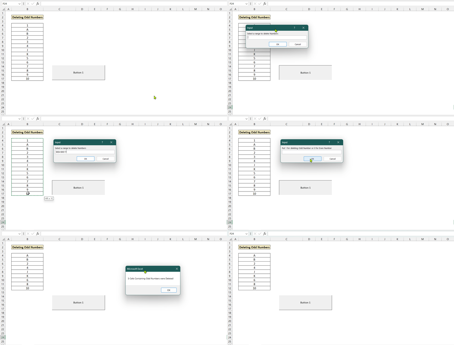
After running the code, an InputBox will ask you to select a range from where you want to delete numbers. Then, another InputBox will appear asking you to input 0 for deleting even numbers and 1 for deleting odd numbers. After inserting the number, the cells containing even/odd numbers will be deleted based on your input. I hope the code solves your problem. If you have any further queries, feel free to comment.
Gracias César por tu consulta. Lamentablemente, no podemos seleccionar varias opciones en un ComboBox. Sin embargo, si necesita seleccionar varias opciones, puede utilizar el ListBox que tiene la propiedad MultiSelect. Pero un inconveniente de ListBox es que no permite a los usuarios escribir directamente en él. Para obtener más información sobre MultiSelect ListBox, puede leer este artículo.
Saludos
Aniruddah
Equipo Exceldemy
[Thanks Cesar for your query. Unfortunately, we can not select multiple options in a ComboBox. However, if you need to select multiple options, you can use the ListBox that has the MultiSelect property. But, one drawback of ListBox is that it doesn’t allow the users to directly write on it. To learn more about MultiSelect ListBox, you can read this article.
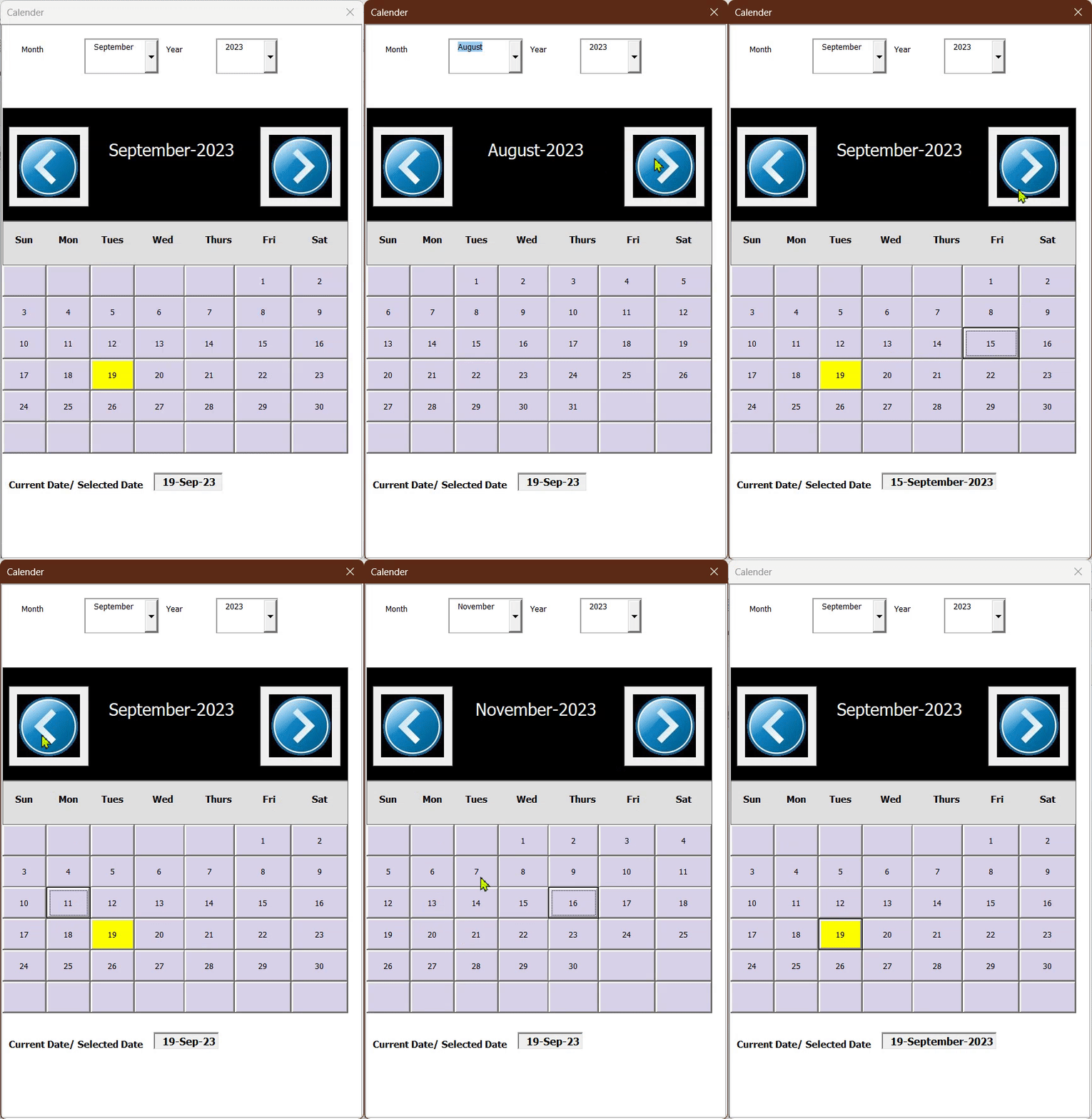
Thanks a lot, MATT, for your comment. If you want to insert a Text Box that will display the current date, and highlight the current date, follow the steps below:
First, draw a Textbox, rename it as “TextBox1”.
You can also insert a Label to show what the Textbox will contain.
Next, go to the D_Col subroutine and modify it in this way:
Sub D_Col()
Dim C_Month As Integer
Dim C_Date As MSForms.CommandButton
For C_Month = 1 To 42
Set C_Date = Me.Controls("CommandButton" & C_Month)
C_Date.BackColor = VBA.RGB(217, 210, 233)
C_Date.Enabled = True
Next C_Month
'Initializing the Textbox with current date
Me.TextBox1.Value = Date
'Highlighting the current date
For i = 1 To 41
Dim cb As CommandButton
Set cb = Me.Controls("CommandButton" & i)
If cb.Caption = Day(Date) And Me.Cmb_Month.Value = VBA.Format(VBA.Date, "MMMM") And Me.Cmb_Year.Value = VBA.Format(VBA.Date, "YYYY") Then
cb.BackColor = vbYellow 'Making it yellow
End If
Next i
End Sub
As whenever any change happens in the userform, this D_Col subroutine is called, so it will always highlight the current date and populate the TextBox1 with the current date.
If you want to populate the TextBox1 with the date of the clicked commandbutton, you need to write event driven subs CommandButton_Click for each of the CommandButtons from CommandButton1 to CommandButton42. Below, I am only giving the CommandButton1_Click sub.
Private Sub CommandButton1_Click()
Dim btn As CommandButton
Set btn = Me.ActiveControl
Date_text = btn.Caption & "-" & Cmb_Month.Text & "-" & Cmb_Year.Text
Me.TextBox1.Text = Date_text
End Sub
You just need to replace the CommandButton1 with CommandButton2, CommandButton3 and so on for the rest of the CommandButtons.
Now, if you run the UserForm, you will get your desired features.
Thanks, GENE for your comment. As you mentioned in your comment, RagTime is a specialized publishing tool with advanced layout and design capabilities. It may be a better choice for complex design and layout requirements for your mail merge documents. If you’re comfortable with a specialized tool, RagTime is a good option. However, if your needs are simple and you’re already familiar with Excel, using it for mail merging can be practical and efficient. So overall it depends on your requirements and in which platform you are used to do your work.
Thank you CANER for your queries.
1. If you want to create a list for only visible sheets, you need to modify the Worksheet_Activate() subroutine in the following way:
Private Sub Worksheet_Activate()
Dim Sheet_Name As Worksheet
Me.Sheet_List.Clear
For Each Sheet_Name In ThisWorkbook.Sheets
'only taking visible sheet in the list
If Sheet_Name.Visible = xlSheetVisible Then
Me.Sheet_List.AddItem Sheet_Name.Name
End If
Next Sheet_Name
End Sub
Here, I have added an extra IF statement so that the code only adds the sheets that are visible to the list.
2. If you want to choose the printer before printing, you need to modify the print_specific_sheets subroutine in the following way:
Sub print_specific_sheets()
Dim n As Long, m As Long
Dim array_1() As Variant
m = 0
With ActiveSheet.Sheet_List
If .ListCount = 0 Then
MsgBox "No Sheet Selected"
Exit Sub
End If
For n = 0 To .ListCount - 1
If .Selected(n) Then
ReDim Preserve array_1(m)
array_1(m) = .List(n)
m = m + 1
End If
Next n
'Opening Printer Setup Dialogue box
Application.Dialogs(xlDialogPrinterSetup).Show
Sheets(array_1()).PrintOut
End With
End Sub
Here, I only added the following line to show the Printer Setup dialogue box from where you can choose from available printers.
Thank you, MATTHEW, for bringing this issue to our attention. After examining the problem, we’ve also identified that the VBA function is not accurately translating the data on Mac OS. You have rightly indicated that the discrepancy in ANSI character codes between Windows and Mac operating systems is the root cause of this problem. We also found that certain characters, such as the initial and final characters Ì and Î, have different codes on Mac and Windows systems. We’re actively working on creating a new VBA function that will function correctly on Mac too.
Thanks Ula, for reaching us out. From your comment, what I can understand is that you have Frequency in one column, Unit time in another column, and you want to covert the total hours (Frequency*Time) to working days. Here, I have prepared a dataset similar to your’s need. I consider the average working hours per day to be 8 and put it in cell D4.
Now, to convert the hours to Workdays, we use the following formula =QUOTIENT(B7*C7,$D$4)&” Days “&((B7*C7/$D$4)-QUOTIENT(B7*C7,$D$4))*$D$4&” Hours”
Here, we used the 4th method of this article where the QUOTIENT function is used. But there are some modifications in the formula. They are described below: B7*C7 is the total hours worked. QUOTIENT(B7*C7,$D$4) returns the total whole working days. ((B7*C7/$D$4)-QUOTIENT(B7*C7,$D$4))*$D$4& returns the remainder extra hours.
Please remember to use absolute reference to the cell Avg. Workday in Hours cell. Then, you can autofill the rest of the cells.
I hope it helps.
Sincerely,
Aniruddah
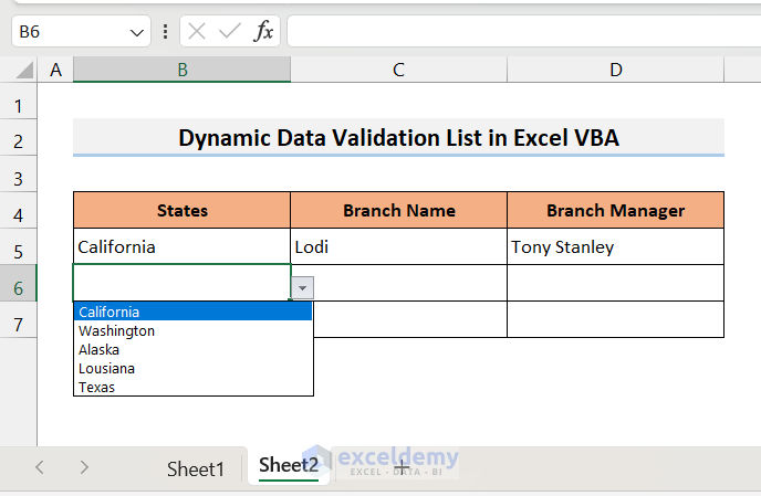
Thank you, WAFEE for reaching out. If your validation list is in a separate sheet, then you need to modify the code in the following way. Follow the steps below.
• First, open a new module and insert the following code in the module.
Sub Update_DataValidation()
Dim sourceSheet As Worksheet
Dim targetSheet As Worksheet
Dim sourceRange As Range
Dim targetRange As Range
Dim lastRow As Long
' Set the source and target sheets
Set sourceSheet = Worksheets("Sheet1") ' Change to your source sheet name
Set targetSheet = Worksheets("Sheet2") ' Change to your target sheet name
' Find the last row in the source list, assuming the list is in column B
lastRow = sourceSheet.Cells(sourceSheet.Rows.Count, "B").End(xlUp).Row
' Define the source range
Set sourceRange = sourceSheet.Range("B3:B" & lastRow) ' Assuming data starts from B3
' Define the target range for data validation, assuming the target range starts at B5
Set targetRange = targetSheet.Range("B5:B" & targetSheet.Cells(targetSheet.Rows.Count, "B").End(xlUp).Row + 1)
' Clear existing data validation in the target range
targetRange.Validation.Delete
' Create a dynamic data validation formula
Dim formula As String
formula = "=" & sourceSheet.Name & "!" & sourceRange.Address
' Apply data validation to the target range
With targetRange.Validation
.Add Type:=xlValidateList, AlertStyle:=xlValidAlertStop, Operator:= _
xlBetween, Formula1:=formula
.IgnoreBlank = True
.InCellDropdown = True
.ShowInput = True
.ShowError = True
End With
End Sub
• Next, you need to paste the following event driven code in both Sheet1 and Sheet2 modules.
Private Sub Worksheet_Change(ByVal Target As Range)
If Not Intersect(Target, Range("$B:$B")) Is Nothing Then
Call Update_DataValidation
End If
End Sub
• The above code will call the Update_DataValidation subroutine whenever you change anything to the B column of the respective sheet. Consequently, the Update_DataValidation subroutine will update the validation options.
• For example, I have my source list in column B of Sheet1 starting from B3.
• On the other hand, we want to validate column B, starting from cell B5 in Sheet2.
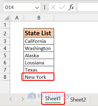
• Now, I add another state to the source list (for example New York).
5-Adding Value in the Source List
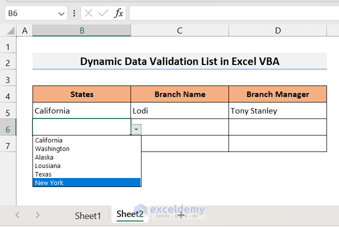
• As soon as I make change in the list, the Update_DataValidation will run in the background. As a result, I also find New York in the validation list in Sheet2.
6-New Item Added in the Validation List
I hope, the codes and example will be helpful to you.
Thank you, Aaron, for your query. To create a drop-down calendar in Microsoft 365 version, you can use the Mini Calendar and Date Picker add-in. To learn how to use the add-in, you can follow this article. I hope, it helps.
Regards
Aniruddah
Thank you Dave for your query. In order to replace the Author with Cell value, in the Extract_All_Comments subroutine, you can replace the following line :
Sub Extract_All_Comments()
Dim wrk_sheet As Worksheet
Dim comm_list As Comment
Dim cal As Long
cal = 0
For Each wrk_sheet In ActiveWorkbook.Worksheets
For Each comm_list In wrk_sheet.Comments
Worksheets("Result").Range("B5").Offset(cal, 0).Parent.Hyperlinks.Add _
Anchor:=Worksheets("Result").Range("B5").Offset(cal, 0), _
Address:="", _
SubAddress:="'" & wrk_sheet.Name & "'!" & comm_list.Parent.Address, _
TextToDisplay:="'" & wrk_sheet.Name & "'!" & comm_list.Parent.Address
Worksheets("Result").Range("C5").Offset(cal, 0).Value = wrk_sheet.Range(comm_list.Parent.Address).Value
Worksheets("Result").Range("D5").Offset(cal, 0).Value = comm_list.Text
cal = cal + 1
Next comm_list
Next wrk_sheet
End Sub
Hope, it will solve your problem.
Regards
Aniruddah
Exceldemy
Thanks MORAN for your query. In order to copy only a number of selected cells(B1, D11, C43) instead of entire UsedRange, you need to modify the code in the following way.
Sub Copy_Selected_cells()
Application.ScreenUpdating = False
Application.EnableEvents = False
Application.Calculation = xlCalculationManual
Sheet_Name = "January" 'Modify this as per your sheet name
Set New_Workbook = ThisWorkbook
Set File_Dialog = Application.FileDialog(msoFileDialogFolderPicker)
File_Dialog.AllowMultiSelect = False
File_Dialog.Title = "Select the Excel Files"
If File_Dialog.Show <> -1 Then
Exit Sub
End If
File_Path = File_Dialog.SelectedItems(1) & "\"
File_Name = Dir(File_Path & "*.xls*")
row_number = 1 'starting from 1st row in Summary Workbook
Do While File_Name <> ""
Set File = Workbooks.Open(Filename:=File_Path & File_Name)
With File.Worksheets(Sheet_Name)
'Copying from Source Sheet and Pasting it on column B(2) in Summary Workbook
.Range("B1").Copy
New_Workbook.Worksheets(Sheet_Name).Cells(row_number, 2).PasteSpecial Paste:=xlPasteAll
'Copying from Source Sheet and Pasting it on column C(3) in Summary Workbook
.Range("D11").Copy
New_Workbook.Worksheets(Sheet_Name).Cells(row_number, 3).PasteSpecial Paste:=xlPasteAll
'Copying from Source Sheet and Pasting it on column D(4) in Summary Workbook
.Range("C43").Copy
New_Workbook.Worksheets(Sheet_Name).Cells(row_number, 4).PasteSpecial Paste:=xlPasteAll
End With
row_number = row_number + 1
File_Name = Dir()
Loop
End Sub
By running the above code, you will be able to extract only selected cells from the source files and paste them on their corresponding columns in the summary file. On the summary file, each row will contain data from a specific file. In the example below, I have extracted B1, D11, C43 cells from 2017,2018 and 2019 files and paste them in column B, C and D respectively.
I hope, this addresses your problem.
Regards
Aniruddah
Thank you GLENN for bringing the issue you faced to our attention. We are sorry to hear that you faced the problem regarding the position of new entries. We have updated the code and Excel file. In the revised code, we have hard-coded the Top_Cell as cell B2 in CommandButton1_Click() subroutine. So make sure that, the headings start at B2 in all the worksheets. Now, you can download the new file and try it again. Hopefully, you will not face the problem anymore.
Sincerely,
Aniruddah
Exceldemy
Hello ANA, Thank you for reaching out to us. We understand that you were previously able to generate emails successfully, but now when running the macro, Outlook does not open with all the information as before.
To identify the problem, it’s challenging to determine the exact cause from here. However, one possibility could be that your deadlines may not have been updated correctly, causing the following lines of code to not execute as expected:
If CDate(xValDateRng) - Date <= 7 And CDate(xValDateRng) - Date > 0 Then
xValSendRng = XRcptsEmail.Offset(k - 1).Value
As you can see, emails will only be sent when the deadline is 7 days or less from the current date. If your deadlines fall within this range and you’re still experiencing issues, we recommend sharing your file with us through the Exceldemy Forum. This will allow us to directly analyze the problem and provide appropriate solutions. Thank you for your cooperation.
Regards
Aniruddah
Thank you for your comment, ROTTIEMOM. Unfortunately, Excel lacks a feature that allows the complete disabling of scientific notation for the entire workbook. In addition to that, when numbers are formatted as Numbers in Excel, there is a maximum limit of 15 digits. If a number exceeds this limit, it will be truncated and displayed in scientific notation, with any digits beyond the 15th being replaced with zeros. To resolve this issue, you have two options: 1)Add an apostrophe (‘) before entering the numbers to treat them as text.
2)Format the cells as text beforehand and then input the numbers in those cells.
Thank you for your comment, MATT D. Unfortunately, Excel lacks a feature that allows the complete disabling of scientific notation for the entire workbook. In addition to that, when numbers are formatted as Numbers in Excel, there is a maximum limit of 15 digits. If a number exceeds this limit, it will be truncated and displayed in scientific notation, with any digits beyond the 15th being replaced with zeros. To resolve this issue, you have two options: 1)Add an apostrophe (‘) before entering the numbers to treat them as text.
2)Format the cells as text beforehand and then input the numbers in those cells.
Thanks for your inquiry. Typically, the “runtime error 9 subscript out of range” occurs when we refer to something that doesn’t exist. In this particular situation, it seems that you haven’t created a worksheet called “January” in the workbook where you’re executing the code. To resolve this, kindly ensure that you create a worksheet with the exact name assigned to the Sheet_Name variable in the code. Once done, you can proceed with running the code, and hopefully, you won’t encounter any issues.
Thanks, SOME, for sharing your problem with us. If you have already tried every method described above, you can try tochange the margin of the page or you can decrease the font size to see if it works for you. If your problem still persists, then I recommend posting your issue and sharing your file on our Exceldemy Forum. This way, we can examine your problem and work towards resolving it.
Regards
Aniruddah
Thanks, LOKESH for your query. In Excel, if you want to convert different date formats into a specific date format with a single formula, the formula will be rather long and complicated. However, you can create a custom function using the following VBA code to do your task.
Code Syntax:
Function FormatDate(cell As Range)
Value = cell.Value
If IsDate(Value) Then
FormatDate = Format(Value, "dd mmm yyyy")
ElseIf Len(Value) = 5 Then
Value = DateSerial(Right(Value, 2) + 2000, Mid(Value, 2, 2), Left(Value, 1))
FormatDate = Format(Value, "dd mmm yyyy")
ElseIf Len(Value) = 6 Then
Value = DateSerial(Right(Value, 2) + 2000, Mid(Value, 3, 2), Left(Value, 2))
FormatDate = Format(Value, "dd mmm yyyy")
ElseIf Len(Value) = 7 Then
Value = DateSerial(Right(Value, 4), Mid(Value, 2, 2), Left(Value, 1))
FormatDate = Format(Value, "dd mmm yyyy")
ElseIf Len(Value) = 8 Then
x = DateSerial(Right(Value, 4), Mid(Value, 3, 2), Left(Value, 2))
If Year(x) < 1900 Then
x = DateSerial(Left(Value, 4), Mid(Value, 5, 2), Right(Value, 2))
End If
FormatDate = Format(x, "dd mmm yyyy")
Else
FormatDate = "Format Not recognised"
End If
End Function
Here, I have created a Custom Function named FormatDate. Then, I apply the function to different date formats that you provided. Here is the result.
Hopefully, it will solve your problem. If you face problems anymore, feel free to post them on our Exceldemy Forum.
Regards
Aniruddah
Thank you for your inquiry, INGE. It is not really clear from your inquiry what you want. I believe you want to know how we can calculate the running total when a month’s entry is zero. In that situation, the Pivot table will add 0 to the previous running total, displaying the same prior running total as before. I hope this clarifies your concerns. If you have any further queries or wish to share your documents, please post them on our Exceldemy Forum (https://exceldemy.com/forum/).
Regards
Aniruddah
Hello, Elena.
Thank you for your kind words. Now, what I can understand from your query is that when you navigate through the preview results, you can only see just one individual’s information rather than everyone’s information. If you exactly follow the steps outlined above, you should be able to see all of the persons’ information in the preview result. Hence, I encourage that you carefully follow the instructions outlined above and observe whether or not your problem is resolved. If your issue persists, you can upload your file to our Exceldemy Forum(https://exceldemy.com/forum/). We will do our best to find a solution.
Thank you Heidi for your comment. You can paste the following VBA code into your Desired Worksheet on the VBA window. This code will automatically update the current date in the corresponding cell of column N if anything is changed in columns O:V. Hope, it will solve your problem. If you have any further queries, you can post them on our Exceldemy Forum.
Regards
Aniruddah
Team Exceldemy
Private Sub Worksheet_Change(ByVal Target As Range)
Dim cell As Range
If Not Intersect(Target, Range("O:V")) Is Nothing Then
For Each cell In Intersect(Target, Range("O:V")).Cells
If cell.Row <= 400 Then
Range("N" & cell.Row).Value = Date
End If
Next cell
End If
End Sub
Thank you JIGNESH for reaching out. Here is a VBA Macro code that will take “To Email Address”, “Email ID CC”, “Subject”, and “Date” ranges from the user and if the code finds any Date which is greater than the Current Date, an email will be sent to the corresponding mail address and CC address with corresponding Subject line. If you have any further queries, feel free to post on our ExcelDemy Forum.
Regards
Aniruddah
Public Sub SendEmailWhenDue()
Dim Date_Range, Mail_Cc, Mail_Subject As Range
Dim Mail_Recipient As Range
Dim Email_Text As Range
Dim Outlook_App_Create As Object
Dim Mail_Item As Object
Dim Last_Row As Long
Dim VB_CR_LF, Email_Body, Date_Range_Value, Send_Value, Subject As String
Dim i As Long
Set Date_Range = Application.InputBox("Please choose the date range:", "Insert Date Range", Type:=8)
If Date_Range Is Nothing Then Exit Sub
Set Mail_Recipient = Application.InputBox("Please select the range of Email addresses:", "Insert Mail Recipeint", Type:=8)
If Mail_Recipient Is Nothing Then Exit Sub
Set Mail_Cc = Application.InputBox("Please choose the CC range:", "Insert CC Range", Type:=8)
Set Mail_Subject = Application.InputBox("Please choose the Subject range:", "Insert Date Range", Type:=8)
Last_Row = Date_Range.Rows.Count
Set Date_Range = Date_Range(1)
Set Mail_Recipient = Mail_Recipient(1)
Set Mail_Cc = Mail_Cc(1)
Set Mail_Subject = Mail_Subject(1)
Set Outlook_App_Create = CreateObject("Outlook.Application")
For i = 1 To Last_Row
Date_Range_Value = ""
Date_Range_Value = Date_Range.Offset(i - 1).Value
If Date_Range_Value <> "" Then 'Condition for sending mail.
If CDate(Date_Range_Value) <= Date Then
Send_Value = Mail_Recipient.Offset(i - 1).Value
Cc = Mail_Cc.Offset(i - 1).Value
Subject = Mail_Subject.Offset(i - 1).Value
Email_Body = " Hi, <br> Please check the reminder." 'Compose your Body Here
Set Mail_Item = Outlook_App_Create.CreateItem(0)
With Mail_Item
.Subject = Subject
.Cc = Cc
.To = Send_Value
.HTMLBody = Email_Body
.Display
End With
Set Mail_Item = Nothing
End If
End If
Next
Set Outlook_App_Create = Nothing
End Sub
Thank you for your query, DUONG. The third, fifth, and seventh approaches mentioned above can be used safely when numerous people share the same mark. However, their rankings on the Top 10 list are based on where they actually stand on the unsorted list. For instance, Jessica, Henderson, and Aaron will be in positions 5, 6, and 7, respectively, in the Top 10 list, if they all receive 70 marks. I believe Hope you got your answer. Please ask on our ExcelDemy forum if you have any additional questions.
Regards
Aniruddah
Thank you Paul for reaching out. For your special case, it is possible to make a custom function that sums up all the numbers within a specific date range and has specific font color. To do this, we have to pass two more arguments in the function (Starting_Date & Ending_Date). For illustration, I have taken another data set that contains Dates on the column header as you suggested.
I have written another code to create a User-defined Function named SumByDateColor.
Function SumByDateColor(starting_date As Variant, ending_date As Variant, ref_color As Range, sum_range As Range) As Double
Dim cell_color As Long, sum_cell As Double
Dim cell As Range
Application.Volatile
sum_cell = 0
cell_color = ref_color.Font.colorIndex
'iterating through columns
For i = 1 To sum_range.Columns.Count
If (sum_range.Cells(1, i) >= starting_date And sum_range.Cells(1, i) <= ending_date) Then
For j = 2 To sum_range.Rows.Count
'iterating through rows from each column
Set cell = sum_range.Cells(j, i)
If cell_color = cell.Font.colorIndex Then
sum_cell = sum_cell + cell.Value
End If
Next j
End If
Next i
SumByDateColor = sum_cell
End Function
In cell L5, if we apply the function, it will return the sum of all the black font numbers from the first three columns (From 03/03/23 to 03/05/23). =SUMBYDateColor(I5,J5,K5,$B$4:$G$10)
In this way, we can apply the function for L6: L9 as well and get the following result.
I hope it will solve your problem. If you have any further queries or need the work file, you can ask in our Exceldemy Forum.
Regards
Aniruddah
Hi Keaton, thanks for your query. As the code has no limitation on the number of rows, it should work in your case. Maybe the code worked for the first 109 rows only because you only selected the first 109 rows in the prompt. Kindly select the entire dataset while running the code. Hopefully, it will do the job for you. If the code still doesn’t work, you can share your file using our Exceldemy forum(https://exceldemy.com/forum/).
Thanks, Janel, for your comment. To find all the data of Emily and Jenifer at once, you can utilize the Filter feature of the Excel table shown in method 4 (Return Multiple Values by Using Excel Defined Table). Here, after clicking the down arrow icon, you need to check both Emily and Jenifer in the filter option to get the hobby list of both persons. Hopefully, it will solve your problem.
Dear Pepijn,
Thank you for sharing your problem. You may be experiencing the same issue as MICHAEL who shared his problem in the comment section above. Please try the solution suggested by Yousuf and let us know if the problem still persists. You can also share your file in our forum for us to investigate the issue closely.
Best of luck.
Regards,
Aniruddah
Hi KOH,
Thanks for reaching out to us! Unfortunately, the method discussed above doesn’t currently support recording half-day leave. We understand how frustrating that can be, and we’re sorry for any inconvenience caused. Rest assured, we’ll definitely work on overcoming this limitation in the future.
We’re grateful for your support of Exceldemy and we hope to make your experience even better in the future.
Best regards,
Aniruddah
Team Exceldemy
Dear Gary,
Thank you for sharing your problem with us. Yes, you are right that when you apply the conditional formatting (color scale) to the entire range,it ranks by each column, not by each row. Hence, in this case, to rank them by rows, you need to apply the conditional formatting to all the rows one by one. I have created a dataset based on your information and applied the conditional formatting to all the rows separately and got the expected result.

If you need to do this kind of stuff frequently, using VBA is indeed the best option as you mentioned.
Regards
Aniruddah
Team Exceldemy
Hi AMR,
Thanks for reaching out! Could you please explain a bit more about what you want to do? I wasn’t able to fully understand your comment. Do you need to get all the permutations? Let us know in the reply.
Regards
Aniruddah
Dear Mary,
You can use the following code that also includes signature.
Feel free to customize the Signature accordingly.
Regards
Aniruddah
Team Exceldemy
Dear DANIELLA,
Thanks for your comment. Have you tried the methods mentioned in this article to solve the issue? If you need further assistance, you can share your file in our Exceldemy Forum (https://exceldemy.com/forum/).
Regards
Aniruddah
Team Exceldemy
Dear Perry,
Thanks for your comment. Unfortunately, Excel does not have a Military time format. However, we can use the custom format feature in Excel to display military time. Follow the steps below to do so:
First, store the military time in text format. I store them as text format in cell C3 and C4 by selecting the cells and selecting “Text” from the Number group on Home tab.
Then, to add the times, use the following formula in cell B4:
=TEXT((TIME(LEFT(C2,2),RIGHT(C2,2),0)+TIME(LEFT(C3,2),RIGHT(C3,2),0)),”hhmm”)
Formula Breakdown:
LEFT(C2,2) and RIGHT(C2,2): Extract the hours and minutes from cell C2.
LEFT(C3,2) and RIGHT(C3,2): Extract the hours and minutes from cell C3.
TIME(…): Create time values for the extracted hours and minutes.
TIME(LEFT(C2,2),RIGHT(C2,2),0)+TIME(LEFT(C3,2),RIGHT(C3,2),0): Add the times
TEXT(…, “hhmm”): Format the time difference as Military Times.
Note: Ensure that cells C2 and C3 are formatted as text to prevent Excel from automatically converting the time values. If Excel interprets them as time values, it may not work as expected. Also, if the total time exceeds 24 hours, it will not return the correct result. To address the issue, we have to create a custom function that requires VBA coding. If this solution does not meet your requirements, you can ask for a a customized solution on our Exceldemy Service.
Regards
Aniruddah
Team Exceldemy
Dear ADAM,
Thanks for your comment. Unfortunately, Excel’s current time formatting does not support metric time display.
Regards
Aniruddah
Team Exceldemy
Dear Slayton,
Thank you for raising a valid concern about preserving text data in Excel. I completely agree that the current limitation, preserving only the upper-left value during a merge, can be frustrating.
To address this, I suggest exploring the five methods mentioned earlier to find the most suitable workaround for your specific case. Additionally, let’s hope that Microsoft Excel considers implementing a new merge option in the future, one that preserves all cell data.
Your feedback is valuable, and we appreciate your engagement.
Best regards,
Aniruddah
Team Exceldemy
Hi Sjoerd,
Thanks for reaching out to us. Unfortunately, Conditional Formatting cannot create a vertical progress bar. But, using Sparkline can help you achieve your goal. You mentioned using Sparkline, but we didn’t understand what you meant by “not the entire range is filled.” Could you please clarify that?
Here’s a sample picture of a vertical progress bar that we created using Sparkline.

Were you referring to the extra space on the two sides of the column, as marked in the picture? If so, we are currently unaware of any methods to eliminate the space. Please let us know your thoughts.
Regards
Aniruddah
Team Exceldemy
Dear Amedeo,
Perhaps you are trying to break the file level protection. Unfortunately, the Zip method can only break the password on worksheet level or workbook level protection. Although this information may not have been highlighted earlier, is now included in a Note.
Regards
Aniruddah
Team Exceldemy
Thanks Nicu for reaching us out. To delete odd or even numbers in a range, you can use the following VBA Code:
After running the code, an InputBox will ask you to select a range from where you want to delete numbers. Then, another InputBox will appear asking you to input 0 for deleting even numbers and 1 for deleting odd numbers. After inserting the number, the cells containing even/odd numbers will be deleted based on your input. I hope the code solves your problem. If you have any further queries, feel free to comment.
Regards
Aniruddah
Team Exceldemy
Gracias César por tu consulta. Lamentablemente, no podemos seleccionar varias opciones en un ComboBox. Sin embargo, si necesita seleccionar varias opciones, puede utilizar el ListBox que tiene la propiedad MultiSelect. Pero un inconveniente de ListBox es que no permite a los usuarios escribir directamente en él. Para obtener más información sobre MultiSelect ListBox, puede leer este artículo.
Saludos
Aniruddah
Equipo Exceldemy
[Thanks Cesar for your query. Unfortunately, we can not select multiple options in a ComboBox. However, if you need to select multiple options, you can use the ListBox that has the MultiSelect property. But, one drawback of ListBox is that it doesn’t allow the users to directly write on it. To learn more about MultiSelect ListBox, you can read this article.
Regards
Aniruddah
Team Exceldemy]
Thanks a lot, MATT, for your comment. If you want to insert a Text Box that will display the current date, and highlight the current date, follow the steps below:
First, draw a Textbox, rename it as “TextBox1”.
You can also insert a Label to show what the Textbox will contain.
Next, go to the D_Col subroutine and modify it in this way:
As whenever any change happens in the userform, this D_Col subroutine is called, so it will always highlight the current date and populate the TextBox1 with the current date.
If you want to populate the TextBox1 with the date of the clicked commandbutton, you need to write event driven subs CommandButton_Click for each of the CommandButtons from CommandButton1 to CommandButton42. Below, I am only giving the CommandButton1_Click sub.
You just need to replace the CommandButton1 with CommandButton2, CommandButton3 and so on for the rest of the CommandButtons.
Now, if you run the UserForm, you will get your desired features.
Here, I am attaching the Excel File with modified UserForm and VBA Codes :VBA UserForm Calender.xlsm
Thanks, GENE for your comment. As you mentioned in your comment, RagTime is a specialized publishing tool with advanced layout and design capabilities. It may be a better choice for complex design and layout requirements for your mail merge documents. If you’re comfortable with a specialized tool, RagTime is a good option. However, if your needs are simple and you’re already familiar with Excel, using it for mail merging can be practical and efficient. So overall it depends on your requirements and in which platform you are used to do your work.
Regards
Aniruddah
Team Exceldemy
Thank you CANER for your queries.
1. If you want to create a list for only visible sheets, you need to modify the Worksheet_Activate() subroutine in the following way:
Here, I have added an extra IF statement so that the code only adds the sheets that are visible to the list.
2. If you want to choose the printer before printing, you need to modify the print_specific_sheets subroutine in the following way:
Here, I only added the following line to show the Printer Setup dialogue box from where you can choose from available printers.
I hope it solves your problem.
Regards
Aniruddah
Team Exceldemy
Thank you, MATTHEW, for bringing this issue to our attention. After examining the problem, we’ve also identified that the VBA function is not accurately translating the data on Mac OS. You have rightly indicated that the discrepancy in ANSI character codes between Windows and Mac operating systems is the root cause of this problem. We also found that certain characters, such as the initial and final characters Ì and Î, have different codes on Mac and Windows systems. We’re actively working on creating a new VBA function that will function correctly on Mac too.
Regards
Aniruddah
Team Exceldemy
Thank you LUBIS for reaching us out. You can run the following VBA code to convert all formulas into values across all the sheets in the workbook.
This code utilizes a “For Each” loop to iterate through each worksheet in the workbook.
Regards
Aniruddah
Exceldemy
Thanks Ula, for reaching us out. From your comment, what I can understand is that you have Frequency in one column, Unit time in another column, and you want to covert the total hours (Frequency*Time) to working days. Here, I have prepared a dataset similar to your’s need. I consider the average working hours per day to be 8 and put it in cell D4.
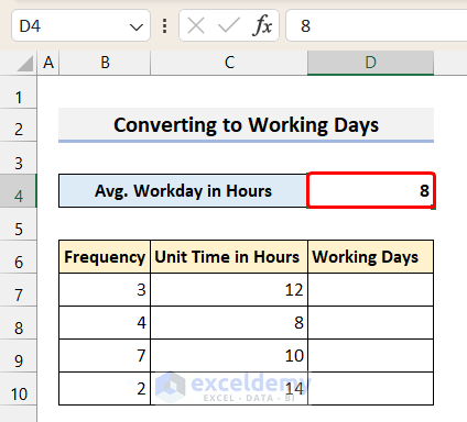
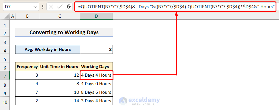
Now, to convert the hours to Workdays, we use the following formula
=QUOTIENT(B7*C7,$D$4)&” Days “&((B7*C7/$D$4)-QUOTIENT(B7*C7,$D$4))*$D$4&” Hours”
Here, we used the 4th method of this article where the QUOTIENT function is used. But there are some modifications in the formula. They are described below:
B7*C7 is the total hours worked.
QUOTIENT(B7*C7,$D$4) returns the total whole working days.
((B7*C7/$D$4)-QUOTIENT(B7*C7,$D$4))*$D$4& returns the remainder extra hours.
Please remember to use absolute reference to the cell Avg. Workday in Hours cell. Then, you can autofill the rest of the cells.
I hope it helps.
Sincerely,
Aniruddah
Thank you, WAFEE for reaching out. If your validation list is in a separate sheet, then you need to modify the code in the following way. Follow the steps below.
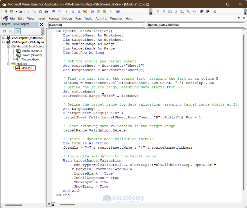
• First, open a new module and insert the following code in the module.
• Next, you need to paste the following event driven code in both Sheet1 and Sheet2 modules.
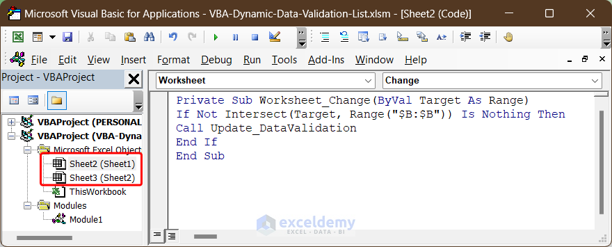
• The above code will call the Update_DataValidation subroutine whenever you change anything to the B column of the respective sheet. Consequently, the Update_DataValidation subroutine will update the validation options.
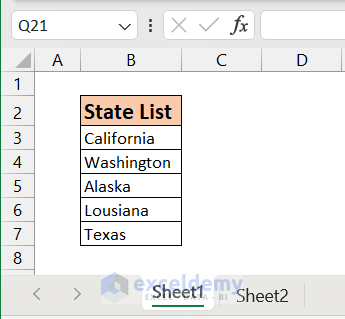
• For example, I have my source list in column B of Sheet1 starting from B3.
• On the other hand, we want to validate column B, starting from cell B5 in Sheet2.
• Now, I add another state to the source list (for example New York).
5-Adding Value in the Source List
• As soon as I make change in the list, the Update_DataValidation will run in the background. As a result, I also find New York in the validation list in Sheet2.
6-New Item Added in the Validation List
I hope, the codes and example will be helpful to you.
Regards
Aniruddah
Thank you, Aaron, for your query. To create a drop-down calendar in Microsoft 365 version, you can use the Mini Calendar and Date Picker add-in. To learn how to use the add-in, you can follow this article. I hope, it helps.
Regards
Aniruddah
Thank you Dave for your query. In order to replace the Author with Cell value, in the Extract_All_Comments subroutine, you can replace the following line :
with this line:
So the final code will be as below:
Hope, it will solve your problem.
Regards
Aniruddah
Exceldemy
Thanks MORAN for your query. In order to copy only a number of selected cells(B1, D11, C43) instead of entire UsedRange, you need to modify the code in the following way.
By running the above code, you will be able to extract only selected cells from the source files and paste them on their corresponding columns in the summary file. On the summary file, each row will contain data from a specific file. In the example below, I have extracted B1, D11, C43 cells from 2017,2018 and 2019 files and paste them in column B, C and D respectively.
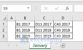
I hope, this addresses your problem.
Regards
Aniruddah
Thank you GLENN for bringing the issue you faced to our attention. We are sorry to hear that you faced the problem regarding the position of new entries. We have updated the code and Excel file. In the revised code, we have hard-coded the Top_Cell as cell B2 in CommandButton1_Click() subroutine. So make sure that, the headings start at B2 in all the worksheets. Now, you can download the new file and try it again. Hopefully, you will not face the problem anymore.
Sincerely,
Aniruddah
Exceldemy
Hello ANA, Thank you for reaching out to us. We understand that you were previously able to generate emails successfully, but now when running the macro, Outlook does not open with all the information as before.
To identify the problem, it’s challenging to determine the exact cause from here. However, one possibility could be that your deadlines may not have been updated correctly, causing the following lines of code to not execute as expected:
As you can see, emails will only be sent when the deadline is 7 days or less from the current date. If your deadlines fall within this range and you’re still experiencing issues, we recommend sharing your file with us through the Exceldemy Forum. This will allow us to directly analyze the problem and provide appropriate solutions. Thank you for your cooperation.
Regards
Aniruddah
Thank you for your comment, ROTTIEMOM. Unfortunately, Excel lacks a feature that allows the complete disabling of scientific notation for the entire workbook. In addition to that, when numbers are formatted as Numbers in Excel, there is a maximum limit of 15 digits. If a number exceeds this limit, it will be truncated and displayed in scientific notation, with any digits beyond the 15th being replaced with zeros. To resolve this issue, you have two options:
1)Add an apostrophe (‘) before entering the numbers to treat them as text.
2)Format the cells as text beforehand and then input the numbers in those cells.
Regards
Aniruddah
Exceldemy
Thank you for your comment, MATT D. Unfortunately, Excel lacks a feature that allows the complete disabling of scientific notation for the entire workbook. In addition to that, when numbers are formatted as Numbers in Excel, there is a maximum limit of 15 digits. If a number exceeds this limit, it will be truncated and displayed in scientific notation, with any digits beyond the 15th being replaced with zeros. To resolve this issue, you have two options:
1)Add an apostrophe (‘) before entering the numbers to treat them as text.
2)Format the cells as text beforehand and then input the numbers in those cells.
Regards
Aniruddah
Exceldemy
Dear STEVEN,
Thanks for your inquiry. Typically, the “runtime error 9 subscript out of range” occurs when we refer to something that doesn’t exist. In this particular situation, it seems that you haven’t created a worksheet called “January” in the workbook where you’re executing the code. To resolve this, kindly ensure that you create a worksheet with the exact name assigned to the Sheet_Name variable in the code. Once done, you can proceed with running the code, and hopefully, you won’t encounter any issues.
Best regards,
Aniruddah
Thanks, SOME, for sharing your problem with us. If you have already tried every method described above, you can try to change the margin of the page or you can decrease the font size to see if it works for you. If your problem still persists, then I recommend posting your issue and sharing your file on our Exceldemy Forum. This way, we can examine your problem and work towards resolving it.
Regards
Aniruddah
Thanks, LOKESH for your query. In Excel, if you want to convert different date formats into a specific date format with a single formula, the formula will be rather long and complicated. However, you can create a custom function using the following VBA code to do your task.
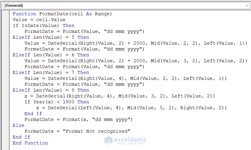
Code Syntax:
Function FormatDate(cell As Range) Value = cell.Value If IsDate(Value) Then FormatDate = Format(Value, "dd mmm yyyy") ElseIf Len(Value) = 5 Then Value = DateSerial(Right(Value, 2) + 2000, Mid(Value, 2, 2), Left(Value, 1)) FormatDate = Format(Value, "dd mmm yyyy") ElseIf Len(Value) = 6 Then Value = DateSerial(Right(Value, 2) + 2000, Mid(Value, 3, 2), Left(Value, 2)) FormatDate = Format(Value, "dd mmm yyyy") ElseIf Len(Value) = 7 Then Value = DateSerial(Right(Value, 4), Mid(Value, 2, 2), Left(Value, 1)) FormatDate = Format(Value, "dd mmm yyyy") ElseIf Len(Value) = 8 Then x = DateSerial(Right(Value, 4), Mid(Value, 3, 2), Left(Value, 2)) If Year(x) < 1900 Then x = DateSerial(Left(Value, 4), Mid(Value, 5, 2), Right(Value, 2)) End If FormatDate = Format(x, "dd mmm yyyy") Else FormatDate = "Format Not recognised" End If End FunctionHere, I have created a Custom Function named FormatDate. Then, I apply the function to different date formats that you provided. Here is the result.
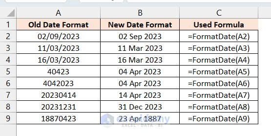
Hopefully, it will solve your problem. If you face problems anymore, feel free to post them on our Exceldemy Forum.
Regards
Aniruddah
Thank you for your inquiry, INGE. It is not really clear from your inquiry what you want. I believe you want to know how we can calculate the running total when a month’s entry is zero. In that situation, the Pivot table will add 0 to the previous running total, displaying the same prior running total as before. I hope this clarifies your concerns. If you have any further queries or wish to share your documents, please post them on our Exceldemy Forum (https://exceldemy.com/forum/).
Regards
Aniruddah
Hello, Elena.
Thank you for your kind words. Now, what I can understand from your query is that when you navigate through the preview results, you can only see just one individual’s information rather than everyone’s information. If you exactly follow the steps outlined above, you should be able to see all of the persons’ information in the preview result. Hence, I encourage that you carefully follow the instructions outlined above and observe whether or not your problem is resolved. If your issue persists, you can upload your file to our Exceldemy Forum(https://exceldemy.com/forum/). We will do our best to find a solution.
Thank you Heidi for your comment. You can paste the following VBA code into your Desired Worksheet on the VBA window. This code will automatically update the current date in the corresponding cell of column N if anything is changed in columns O:V. Hope, it will solve your problem. If you have any further queries, you can post them on our Exceldemy Forum.
Regards
Aniruddah
Team Exceldemy
Thank you JIGNESH for reaching out. Here is a VBA Macro code that will take “To Email Address”, “Email ID CC”, “Subject”, and “Date” ranges from the user and if the code finds any Date which is greater than the Current Date, an email will be sent to the corresponding mail address and CC address with corresponding Subject line. If you have any further queries, feel free to post on our ExcelDemy Forum.
Regards
Aniruddah
Thank you for your query, DUONG. The third, fifth, and seventh approaches mentioned above can be used safely when numerous people share the same mark. However, their rankings on the Top 10 list are based on where they actually stand on the unsorted list. For instance, Jessica, Henderson, and Aaron will be in positions 5, 6, and 7, respectively, in the Top 10 list, if they all receive 70 marks. I believe Hope you got your answer. Please ask on our ExcelDemy forum if you have any additional questions.
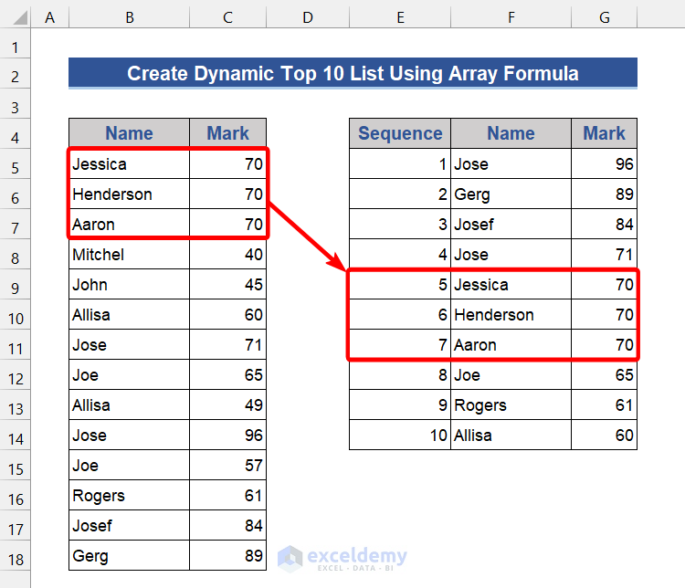
Regards
Aniruddah
Thank you Paul for reaching out. For your special case, it is possible to make a custom function that sums up all the numbers within a specific date range and has specific font color. To do this, we have to pass two more arguments in the function (Starting_Date & Ending_Date). For illustration, I have taken another data set that contains Dates on the column header as you suggested.
I have written another code to create a User-defined Function named SumByDateColor.
In cell L5, if we apply the function, it will return the sum of all the black font numbers from the first three columns (From 03/03/23 to 03/05/23).
=SUMBYDateColor(I5,J5,K5,$B$4:$G$10)In this way, we can apply the function for L6: L9 as well and get the following result.
I hope it will solve your problem. If you have any further queries or need the work file, you can ask in our Exceldemy Forum.
Regards
Aniruddah
Hi Keaton, thanks for your query. As the code has no limitation on the number of rows, it should work in your case. Maybe the code worked for the first 109 rows only because you only selected the first 109 rows in the prompt. Kindly select the entire dataset while running the code. Hopefully, it will do the job for you. If the code still doesn’t work, you can share your file using our Exceldemy forum(https://exceldemy.com/forum/).
Thanks, Janel, for your comment. To find all the data of Emily and Jenifer at once, you can utilize the Filter feature of the Excel table shown in method 4 (Return Multiple Values by Using Excel Defined Table). Here, after clicking the down arrow icon, you need to check both Emily and Jenifer in the filter option to get the hobby list of both persons. Hopefully, it will solve your problem.