How to Create Multi Select ListBox in Excel (With Easy Steps)

When we work on a large dataset, often it gets difficult to fetch any selective value from it. Moreover, you cannot choose more than multiple pieces of information simultaneously. In this case, ListBox is a very helpful solution in Excel. But the process of creating this ListBox is a bit tricky. Therefore, in this article, we will learn how to create a multi-select ListBox in Excel with some simple steps.

To make the process easier, we have divided it into 8 steps for better understanding. So, without further delay, let’s hop into the steps below to see how we can create a multi-select ListBox in Excel.

Step 1: Creating Excel Table from Dataset

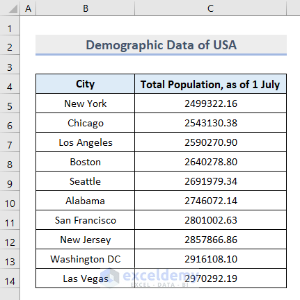
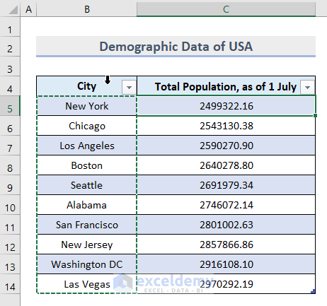
Initially, we need to prepare a sample dataset and convert it into a table. To do this, follow the steps below.

First, create a dataset with the information of 10 City Names and their Total Population of the USA till 1, July in the Cell range B5:C14.

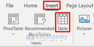
Now, click on any cell of the dataset and choose Table from the Insert tab.

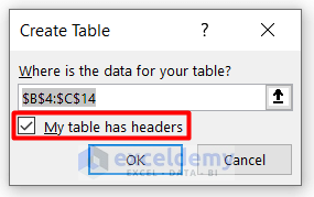
Then, you will see the Create Table window which automatically selects the cell range to create a table.
In this window, mark checked the My table has headers box and press OK.

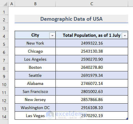
As a result, you will see the dataset is converted to a table.

Along with it, you can find the table in the Table Name box under the Table Design tab

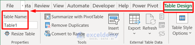
You can change the table name according to your preference.

Step 2: Naming Dataset List from Name Manager

Now, we will name each category of cell range from the table. For this, go through the steps.

First, select any cell from Column B in the table.
Then, go to the Formulas tab and select Define Name.

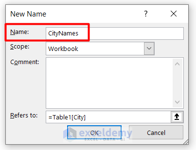
Following this, you will see the New Name dialogue box.
In this dialogue box, provide any name as per the selected column header in the Name box.

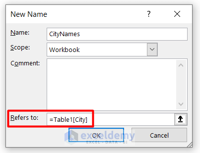
Next, click on the Refers to box in the same window.
Then, put the cursor over the header and it will show a black arrow.
Afterward, press left-click to select the Cell range B5:B14.

As a result, you will see the list of names along with the table name in the Refers to box and press OK.

Follow the same procedure, for the Cell range C5:C14 as well.
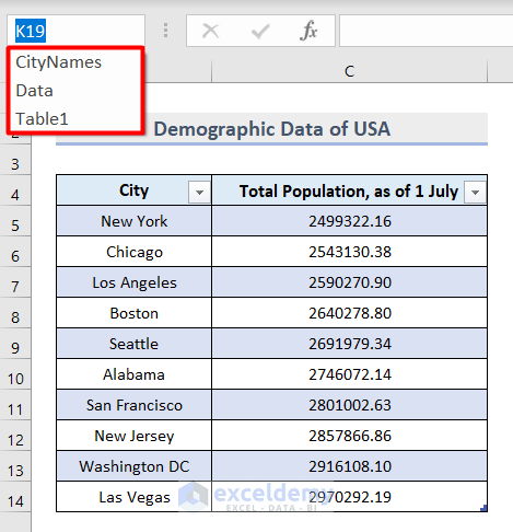
Finally, you will see the names in the Name Box in the upper left corner of the workbook.

Step 3: Creating Drop Down List with Data Validation

At this stage, we will create a drop-down list out of the named ranges with data validation. This is the essential part of creating a ListBox. We will create this in another worksheet in the workbook. But you can do this in the same worksheet as well. Let’s see the process below.

In the beginning, select some cells from the table where you want to apply Data Validation.
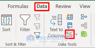
Then, go to the Data tab and choose Data Validation in the Data Tools section.

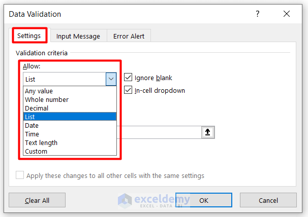
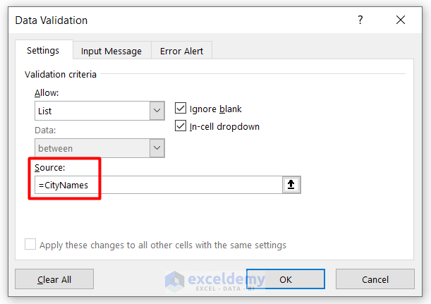
Next, in the Settings tab, choose List in the Allow box.

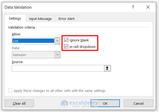
Also, mark checked the Ignore blank and In-cell dropdown boxes.

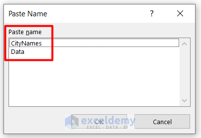
Afterward, click on the Source box in this window and press F3 on your keyboard.
As a result, you will see the Paste Name dialogue box with the name list.
Here, choose CityNames from the list and press OK.

Then, you will see the first list’s name showing in the source box.

Lastly, press OK and apply the same process for the second name list.
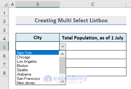
Finally, you will see that Data Validation is activated on the selected cells.

Step 4: Inserting VBA Code to Validated Worksheet

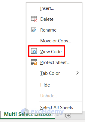
Now comes the crucial part of inserting VBA code to create a ListBox. Following is the process for this.

First, right-click on the validated worksheet and select View Code from the Context Menu.

Then, insert this code on the page.

Private Sub Worksheet_SelectionChange(ByVal Target As Range)
Dim rngDV As Range
Dim oldVal As String
Dim newVal As String
Dim strList As String
On Error Resume Next
Application.EnableEvents = False
   Set rngDV = Cells.SpecialCells(xlCellTypeAllValidation)
   On Error GoTo exitHandler
   If rngDV Is Nothing Then GoTo exitHandler
   If Not Intersect(Target, rngDV) Is Nothing Then
      If Target.Validation.Type = 3 Then
         strList = Target.Validation.Formula1
         strList = Right(strList, Len(strList) - 1)
         strDVList = strList
         frmDVList.Show
      End If
   End If
exitHandler:
  Application.EnableEvents = True
End Sub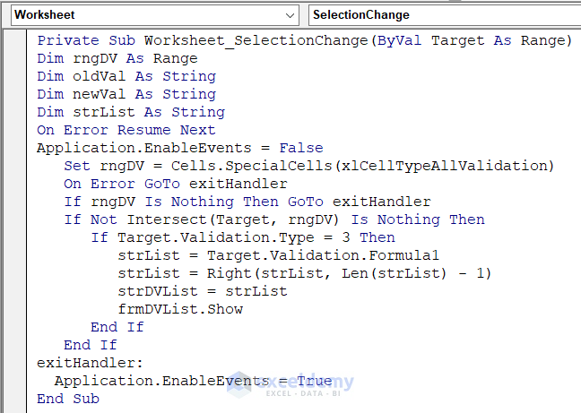

Next, go to the Insert tab and select Module.
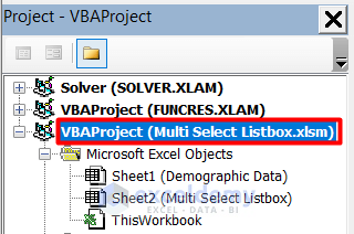
At this point, the workbook name must be selected in the Project Object window.

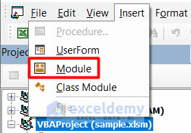
Then, rename the module as modSettings and insert this code.

Option Explicit
Global strDVList As String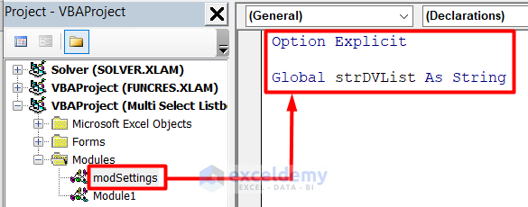

Step 5: Creating UserForm with Listbox & Buttons

At this stage, we will create a UserForm for the workbook along with a ListBox and some Command Buttons. To do this, follow the process below.

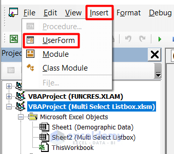
First, select the workbook in the Project-VBAProject window in the Visual Basic editor.

Then, go to the Insert tab and select UserForm.

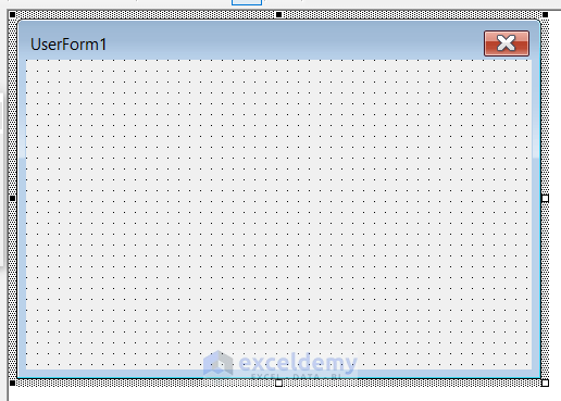
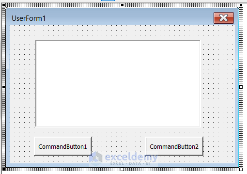
As a result, you will get the UserForm interface like this.

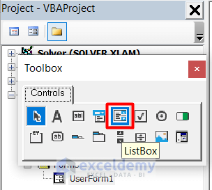
Along with this, you will also get the Toolbox window.
From here, drag ListBox to the UserForm.

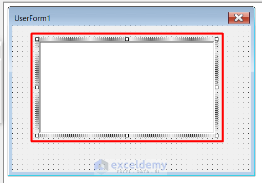
Then, the ListBox will look like this. You can adjust the size by dragging the edges of the box.

Next, drag the CommanButton twice to UserForm as well to create 2 buttons for operation.

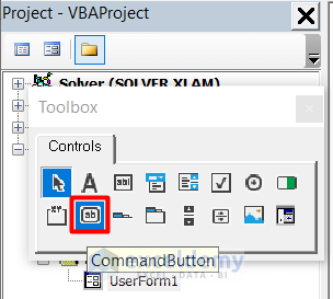
Lastly, the final output looks like this.

Step 6: Changing Settings of Properties

In this stage, we will make some changes in the properties of each component of the ListBox.

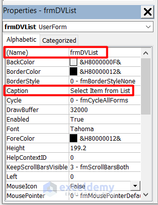
In the beginning, press F4 on the Visual Basic editor to open the Properties Window.
Then, select the UserForm and change the Name and Caption of it like this.

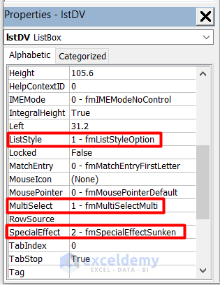
Next, select ListBox and change the Name according to your preference.

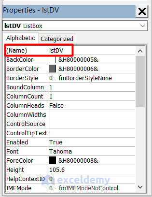
Additionally, change the type of ListStyle, MultiSelect and SpecialEffect as per the image below.

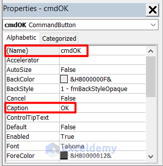
Now, choose the first command button and make the following changes in the properties.

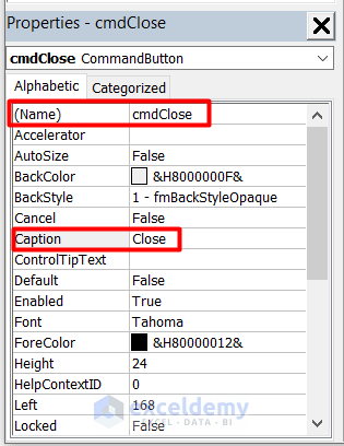
In addition to that, edit the properties of the second command button as well.

Step 7: Applying VBA Code to UserForm

At this stage, we will apply VBA codes to each of the components of the UserForm. Let’s see how it works.

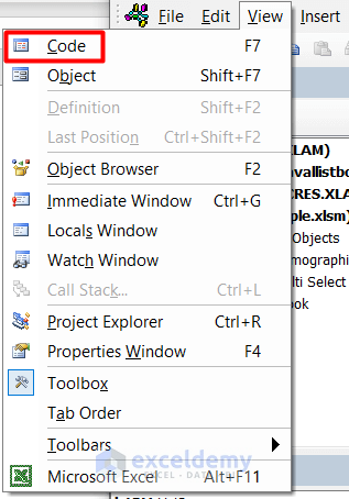
First, select UserForm and go to the View tab to select Code.

Then, insert this code on the blank page. It will automatically run when the UserForm is opened.

Private Sub UserForm_Initialize()
   Me.lstDV.RowSource = strDVList
End Sub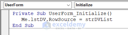

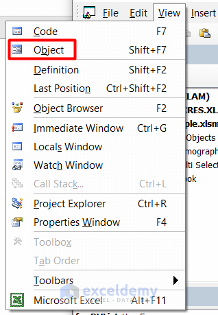
After this, go back to the UserForm interface by clicking on Object on the View tab.

Now, follow the process to insert this code for the OK button.

Private Sub cmdOK_Click()
Dim strSelItems As String
Dim lCountList As Long
Dim strSep As String
Dim strAdd As String
Dim bDup As Boolean
On Error Resume Next
strSep = ", "
With Me.lstDV
   For lCountList = 0 To .ListCount - 1
      If .Selected(lCountList) Then
         strAdd = .List(lCountList)
      Else
         strAdd = ""
      End If
      If strSelItems = "" Then
         strSelItems = strAdd
      Else
         If strAdd <> "" Then
            strSelItems = strSelItems _
              & strSep & strAdd
         End If
      End If
   Next lCountList
End With
With ActiveCell
   If .Value <> "" Then
      .Value = ActiveCell.Value _
        & strSep & strSelItems
   Else
      .Value = strSelItems
   End If
End With
Unload Me
End Sub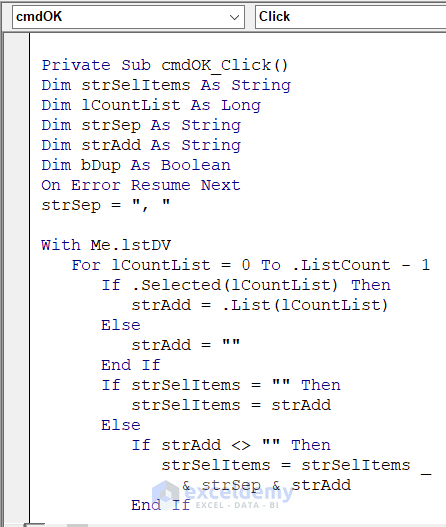

Along with this, type this code for the Close button using the same process.

Private Sub cmdClose_Click()
  Unload Me
End Sub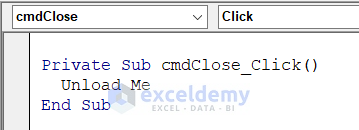

Lastly, press Ctrl + S to save it and close the window.

Step 8: Multi Select from ListBox

Finally, we have successfully created a ListBox for multiple selections. To check if the code is working or not, simply go through these steps.

First, select Cell B5 where we applied Data Validation.
Just right after that, a ListBox will pop-up commanding Select Item from List.
In this window, choose more than one name from the list.

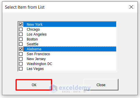
Then, press OK.
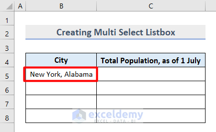
Finally, you have successfully multi-selected from the ListBox and each name is separated by a Comma (,).

Things to Remember

Named ranges will not create a Data Validation rule if they are entered as a cell reference or with delimiters.
The Global variable is applied for both UserForm and Worksheet VBA code. Any active cell name initially passes the code strDVList to a temporary range and then is used as a RowSource for the ListBox when a user opens the UserForm.
You can combine multiple ranges in a single name for ease of selection.

Download Practice Workbook

Get the sample file to practice.

Multi Select ListBox.xlsm

Conclusion

That’s all for today. I hope these long but simple steps on how to create multi select ListBox in Excel have made the topic a little bit easier for you. Let us know your feedback in the comment box.

Get FREE Advanced Excel Exercises with Solutions!

2 Comments

Julie Mar 12, 2022 at 12:47 AM

I’m receiving a “Compile error: Variable not defined” and it’s highlighting “strDVList =”
- Reply
  Tanjima Hossain Aug 30, 2022 at 9:51 AM
  Hello Julie,
  You can try out the following code. I think it will work for you. Just make sure to change the number in Target.Column = 3 according to your column number of data validation.
```
Private Sub Worksheet_Change(ByVal Target As Range)
Dim rngDV As Range
Dim oldVal As String
Dim newVal As String
If Target.Count > 1 Then GoTo exitHandler

On Error Resume Next
Set rngDV = Cells.SpecialCells(xlCellTypeAllValidation)
On Error GoTo exitHandler

If rngDV Is Nothing Then GoTo exitHandler

If Intersect(Target, rngDV) Is Nothing Then
Else
  Application.EnableEvents = False
  newVal = Target.Value
  Application.Undo
  oldVal = Target.Value
  Target.Value = newVal
  If Target.Column = 3 Then
    If oldVal = "" Then
      Else
      If newVal = "" Then
      Else
      Target.Value = oldVal & ", " & newVal

      End If
    End If
  End If
End If

exitHandler:
  Application.EnableEvents = True
End Sub
```