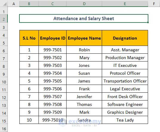
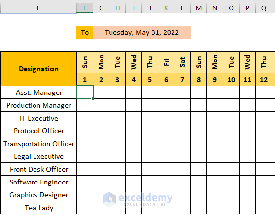
Consider the following information about some employees of an organization. In the dataset, columns C, D, and E contain the data for Employee ID, Employee Name, and Designation.
Step 1 – Put the Name of the Month
We want to create monthly attendance and salary sheet format in Excel. For that, we have to insert the name of the month on the top portion of the format. Follow our steps below:
- Select cell F2.
- Copy the formula below into the cell and press Enter.
=MID(CELL("filename",A1),FIND("]",CELL("filename",A1))+1,255)&" "&2022
Formula Breakdown:
This formula returns the sheet name in the selected cell.
- CELL(“filename”,A1): The CELL function gets the complete name of the worksheet
- FIND(“]”,CELL(“filename”,A1)) +1: The FIND function will give you the position of ] and we’ve added +1 because we require the position of the first character in the name of the sheet.
- 255: Excel’s maximum word count for the sheet name.
- MID: The MID function uses the text’s position from start to end to extract a specific substring.
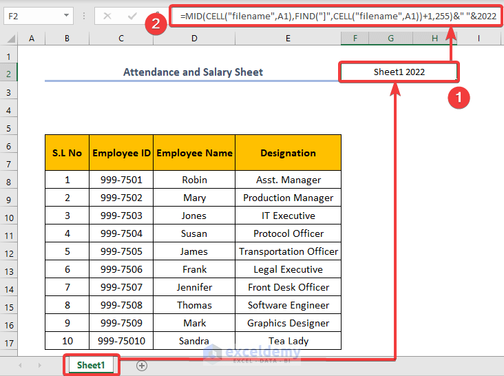
You can see the name of our Sheet on this cell concatenated with 2022.
Note: While using this formula, make sure to enter any cell reference of this sheet. Otherwise, the formula won,t work properly. For example, here we’ve entered the reference of cell A1.
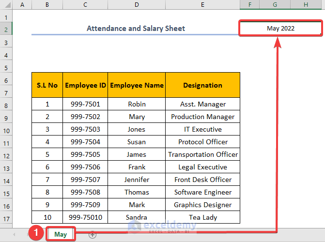
- Change the name of the sheet to May. As we wanna make the attendance sheet of month May’22. We can easily see that the month name is automatically input into cell F2 after changing the sheet name.
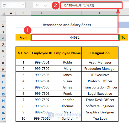
- Set the starting date for this month by selecting cell C4 and inputting the formula below:
=DATEVALUE("1"&F2)
Here, F2 represents the month of May 2022.
A date that is stored as text can be changed into a serial number that Excel can identify as a date using the DATEVALUE function.
Our value comes as a serial number (how Excel stores dates internally). But we want to show it as a date. So, change the format of this cell to Date:
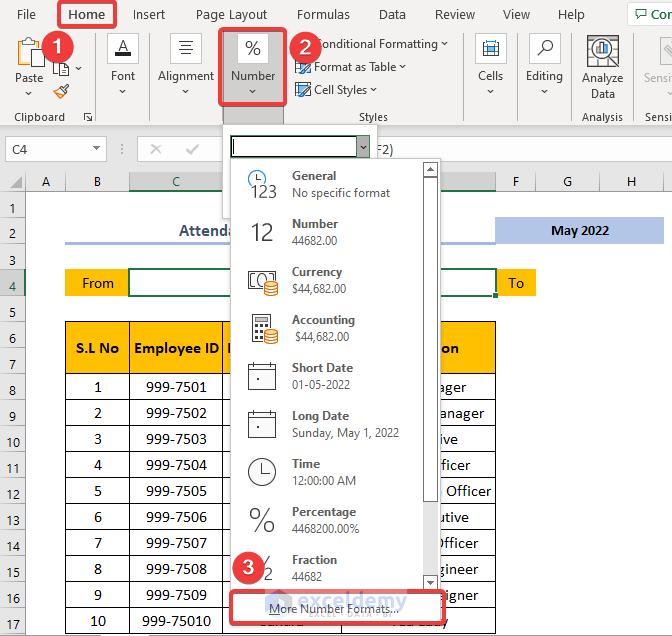
- Select cell C4.
- Go to the Home tab and select Number group.
- Select More Number Formats from the drop-down menu.
- Format Cells dialog box opens. Select Date from Category.
- Choose the following Type (Day of week, Month Day, Year) as the image below and click on OK.
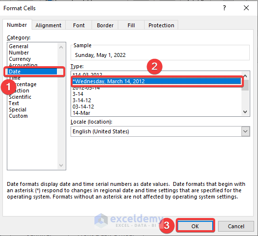
Note: You can press CTRL + 1 to open the Format Cells dialog box.
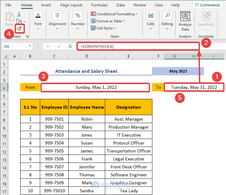
- Select cell G4 to show the ending date of that month. Write down this formula in the cell and press Enter:
=EOMONTH(C4,0)
Here, C4 represents the starting date of the month.
EOMONTH function is used to determine the end of the month. This result will also show in Number format. So, format cell G4 with Format Painter just as cell C4.
Step 2 – Create Individual Date and Day
Follow the steps below:
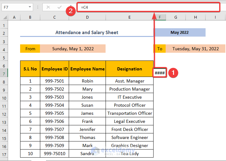
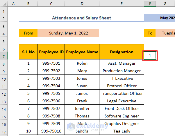
- Select cell F7.
- Type in the formula below and press Enter:
=C4
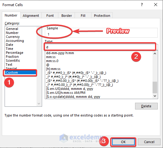
- Press Ctrl + 1 to open the Format Cells wizard.
- Select Custom and type d in the Type box.
- Click on OK.
- At this point, the date should look like the image below.
- Select cell G7.
- Write the formula below and press Enter:.
=IF(F7<$G$4,F7+1,"")
Here, F7 and G4 represent the first date of the month and the last date of the month successively.
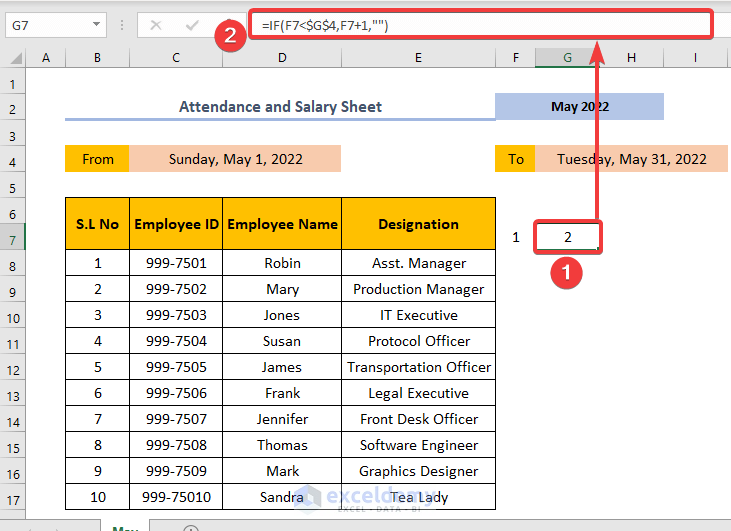
Formula Breakdown:
We’ve applied a logical test using the IF function here. If the date in cell F7 is less than the month’s end date, then the formula returns the next date of the date in cell F7. Otherwise, it will show nothing.
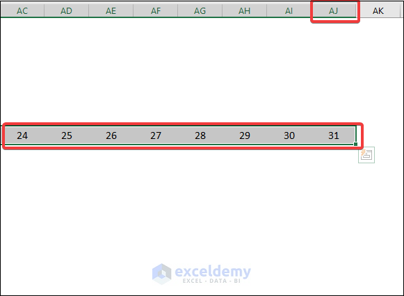
- Use the Fill Handle tool and drag it to cell AJ7 to show the other days of the month.
- Select the columns in the F: AJ range.
- Go to the Home tab.
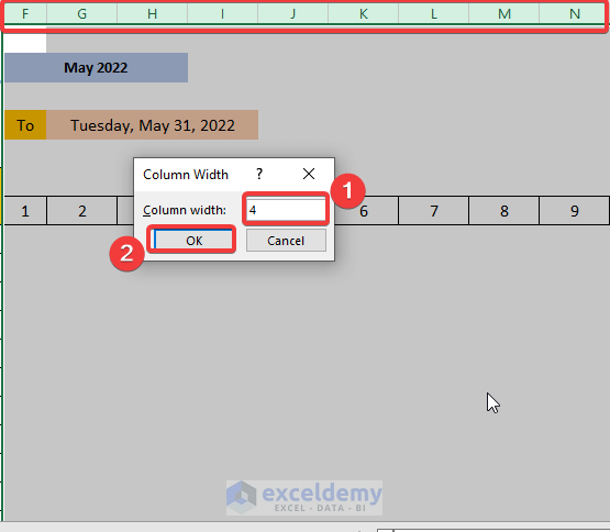
- Select Cells > Format > Column Width.
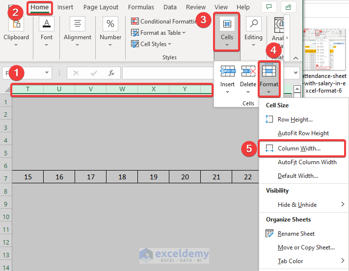
- Type 4 in the Column Width box and click on OK.
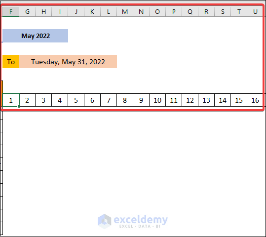
- This is enough to put P or A into these cells.
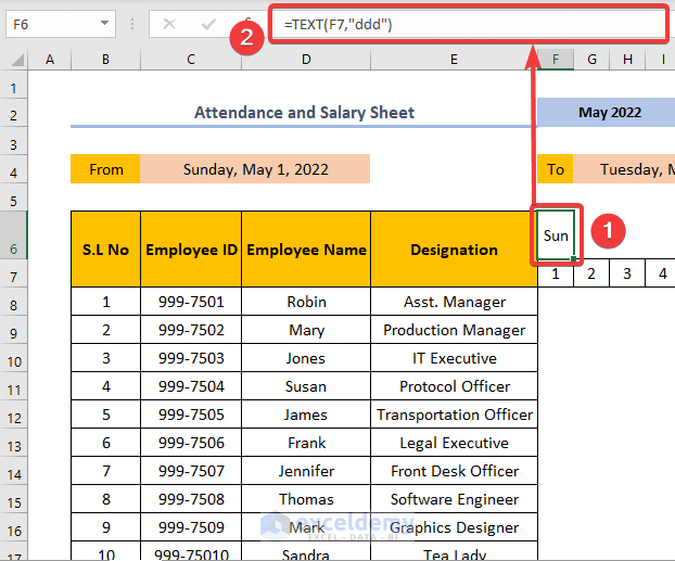
- Select cell F6 and type the formula below.
- Press Enter.
=TEXT(F7,"ddd")
- Fill in the other days using the Fill Handle Tool.
- From the Home tab, click on the small arrow in Alignment group,
- Write down 90 in the Degrees box and click on OK.
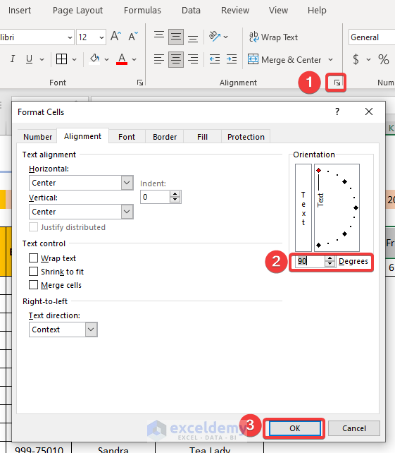
- The name of the days rotates vertically for visibility.
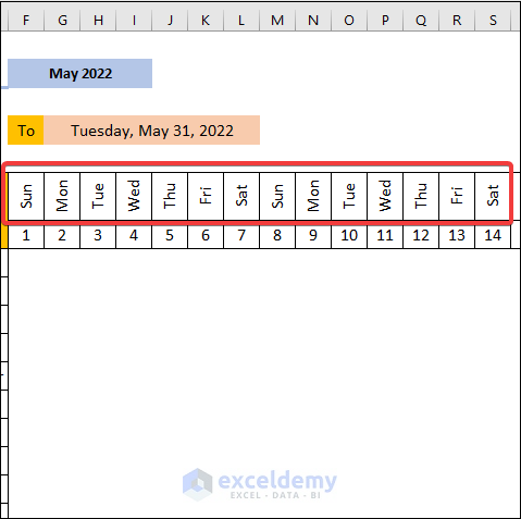
- Fill the cells with your preferred colors and apply All Borders to the cells.
Step 3 – Format Weekly Holidays in Attendance Sheet with Salary Format in Excel
- Select cell F8.
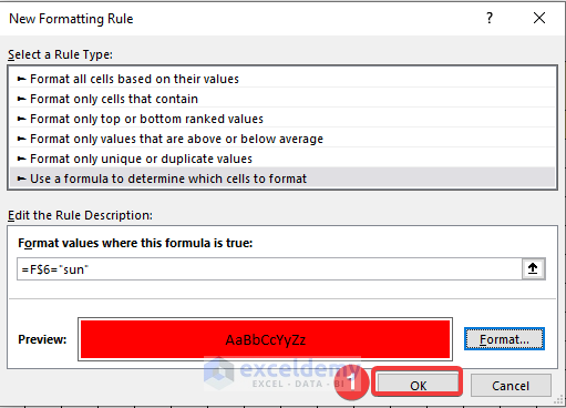
- Go to the Home tab, select Conditional Formatting and go to New Rule.

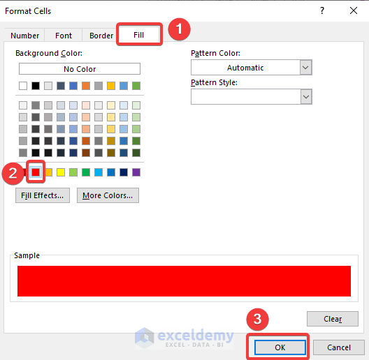
- The New Formatting Rule dialog box will open. Select the “Use a formula…” option (the last one). Write the formula in the formula box and click on Format:
=F$6=”sun”
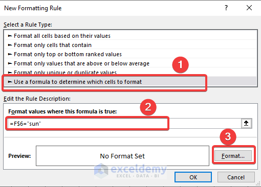
- The Format Cells dialog box opens. Select the Fill tab, choose your preferred color, and click on OK.
- This returns to the New Formatting Rule dialog box. Click on OK to confirm.
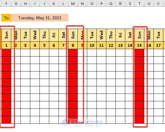
- Use the Fill Handle tool to expand the formatting to all cells in the F8:AJ17 range. The cells under the columns of the Sun are now highlighted. You can repeat the process for Saturday or any other non-working days.
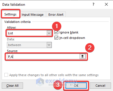
Step 4 – Input Attendance in Cells as P and A
- Select all cells in the F8:AJ17 range.
- Go to the Data tab and select Data Tools, then go to Data Validation.
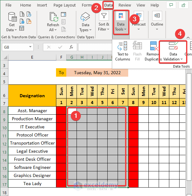
- Go to Settings.
- Select List from the drop-down list in Allow box.
- Write down P, A in the Source box.
- Click on OK.
Here, P means Present, and A means Absent. You can use your own wording but you’ll have to modify the remaining formulas to work around them.
- Click on cell G8.
- You can see a drop-down list containing just P and A. That means those are the only available inputs.
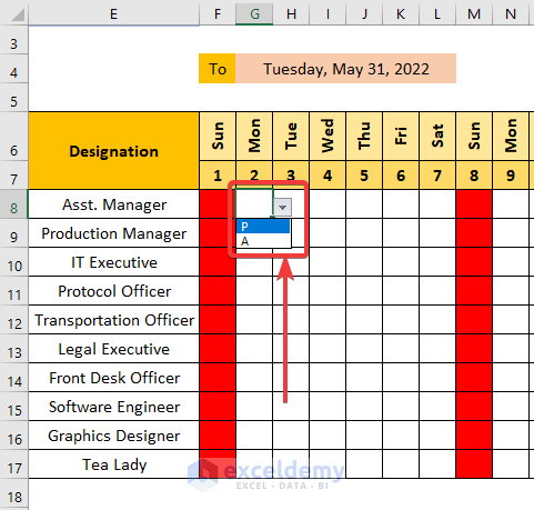
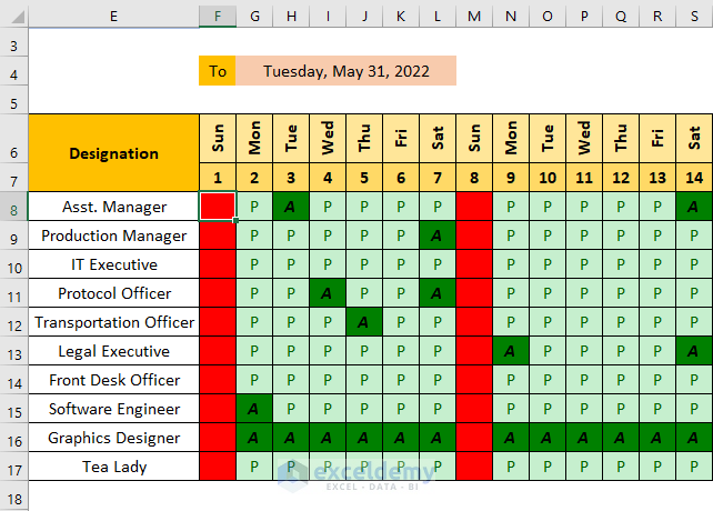
- Fill in the attendance manually. We’ll use the following data as an example.

- Select the cells in the F8:AJ17 range.
- Go to the Home tab.
- Select Conditional Formatting, Highlight Cells Rules, and Text that Contains.
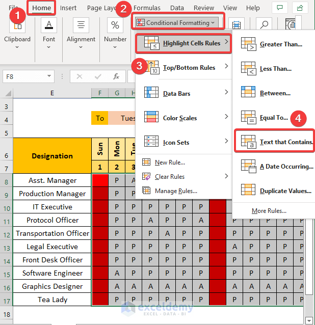
- Write down P in the Format cells that contain the text box.
- Choose the formatting as you like (we used green since P is Present thus positive).
- Click OK.
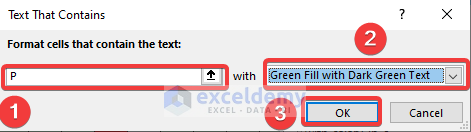
- Cells containing P are now formatted for visibility.
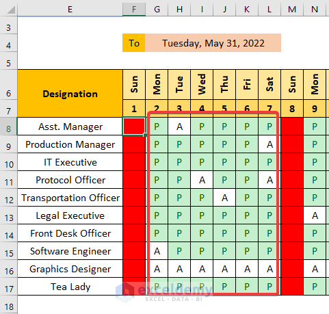
- Format the cells containing A with a different color and formatting.
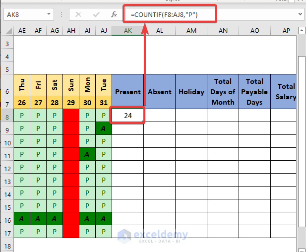
Step 5 – Count Total Payable Days
- Select cell AK8.
- Type the formula below and press Enter:
=COUNTIF(F8:AJ8,"P")
F8:AJ8 represents the cell range to input attendance.
We used the COUNTIF function to count the number of “P”s in the above range.
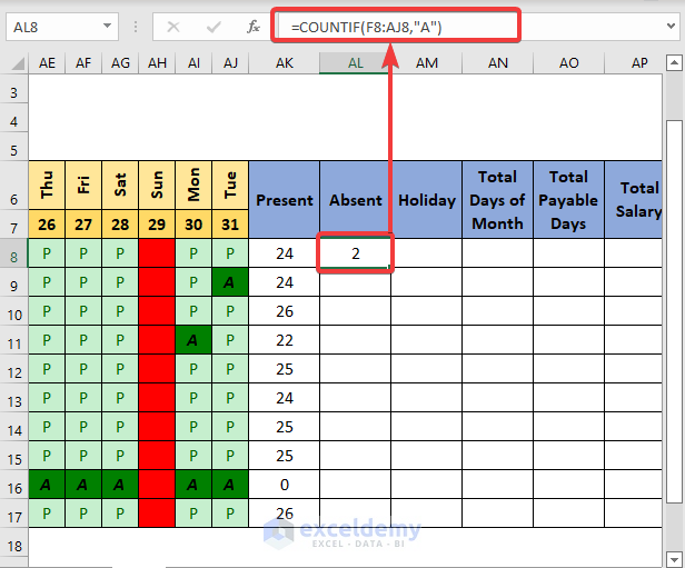
- Select cell AL8.
- Type the formula below and press Enter.
=COUNTIF(F8:AJ8,"A")
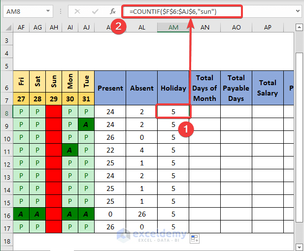
- To calculate the total holidays in the month, select cell AM8. Put the formula below and press Enter. You may need to modify the formula to include other non-working days.
=COUNTIF($F$6:$AJ$6,"sun")
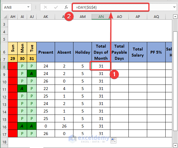
- We can also calculate the Total Days of the Month. Select cell AM8 and write the formula below, then press the Enter key:
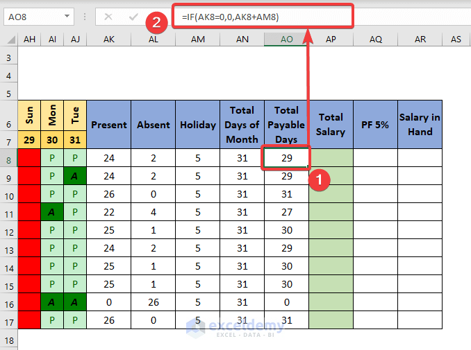
- To calculate Total Payable Days, firstly, select cell AO8. Write down the formula below and press ENTER.
=IF(AK8=0,0,AK8+AM8)
In this place, AK8 and AM8 cells serve as Present Days and Holidays respectively.
Formula Breakdown:
If the number of present days is zero, then the formula returns zero also. That means if an employee becomes absent through the whole month, then he’ll not get paid for the holidays also. Otherwise, he’ll be paid for his present days and weekly holidays.
Step 6 – Calculate Salary in the Attendance Sheet with Salary Format in Excel
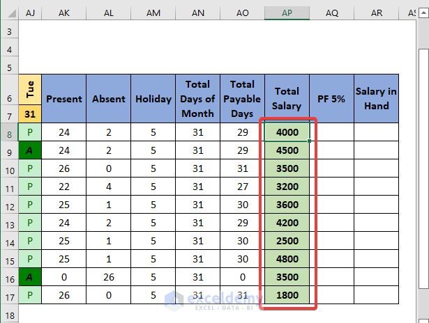
For calculating salary, input the employees’ Total Salary amount.
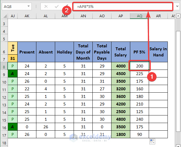
- For this example, here’s a 5% provident fund that is deducted from the Total Salary. For this, select cell AQ8. Write down the formula below and press Enter.
=AP8*5%
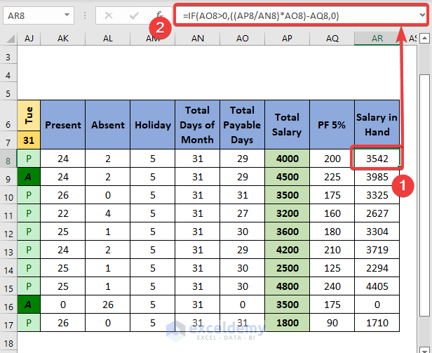
- Finally, to calculate the Salary in Hand, select cell AR8. Type the formula below and press ENTER.
=IF(AO8>0,((AP8/AN8)*AO8)-AQ8,0)
Here, AN8, AO8, AP8, and AQ8 represent Total Days of Month, Total Payable Days, Total Salary, and PF consecutively.
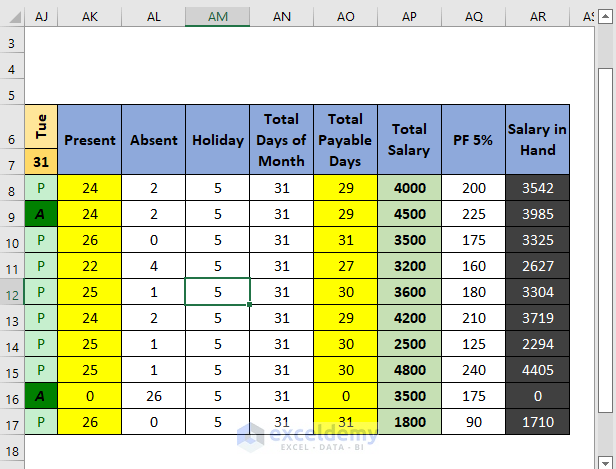
- Format the cells with effective colors to make the data more visible.
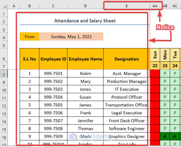
- Use the Freeze Panes tool to freeze the columns in the A:E range and freeze the rows in the 1:7 range.
- Select cell F8 and go to the View tab.
- Select Window group, go to Freeze Panes drop-down menu, and select Freeze Panes.
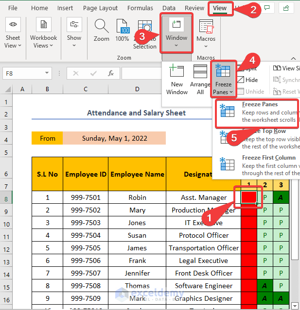
- The cells on left and above F8 are now frozen.
Download Practice Workbook
You may download the following Excel workbook for better understanding and practice yourself.
<< Go Back to Salary | Formula List | Learn Excel
Get FREE Advanced Excel Exercises with Solutions!
