Strikethrough is a special character. It is mainly used to format the cells. When a person applies the strikethrough on any cell, a line appears through the text or the value contained in that cell. Though this is a cell format option, sometimes this option does not remain in the Excel toolbar. In this context, we will demonstrate to you 3 different ways on how to add strikethrough in Excel Toolbar. If you are also interested to know the approaches, download our workbook and follow us.
What Is Strikethrough in Excel?
Strikethrough is a special type of character available in Microsoft Excel. It is a cell format option. After applying the Strikethrough the cell shows a straight line through the cell value. The Strikethrough command in the Excel toolbar shows like the image shown below:

As this feature is a cell format option, sometimes you will find it inside the Font group of the Home tab. The icon is shown below for your convenience.
![]()
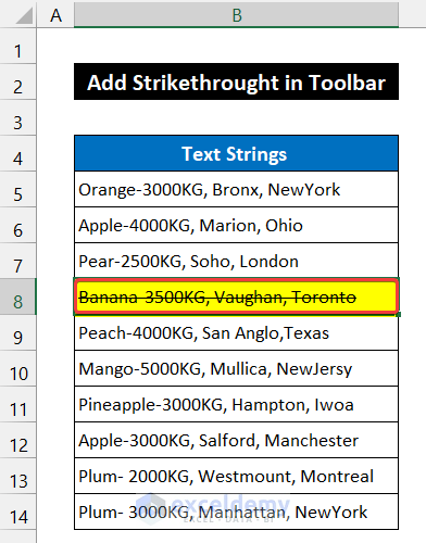
When we apply the strikethrough command to any cell, the cell shows like the image.

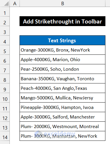
In this context, we will show you 3 distinct methods of adding strikethrough to your Excel spreadsheet toolbar. After adding the command, we will also illustrate its application to our dataset. Regarding that issue, we are considering a dataset of 10 text strings. So, our dataset is in the range of cells B5:B14. We will apply the strikethrough format to cell B8.
1. Using Excel Options to Add Strikethrough in Toolbar
In this following process, we will demonstrate to you how to add the strikethrough command from the Options. The location of this command icon will be inside any existing tab of the Excel toolbar. In our case, we choose the Home tab to allocate the command. The process is explained below as follows:
📌 Steps:
- To enable the Strikethrough command, first of all, select File > Options.
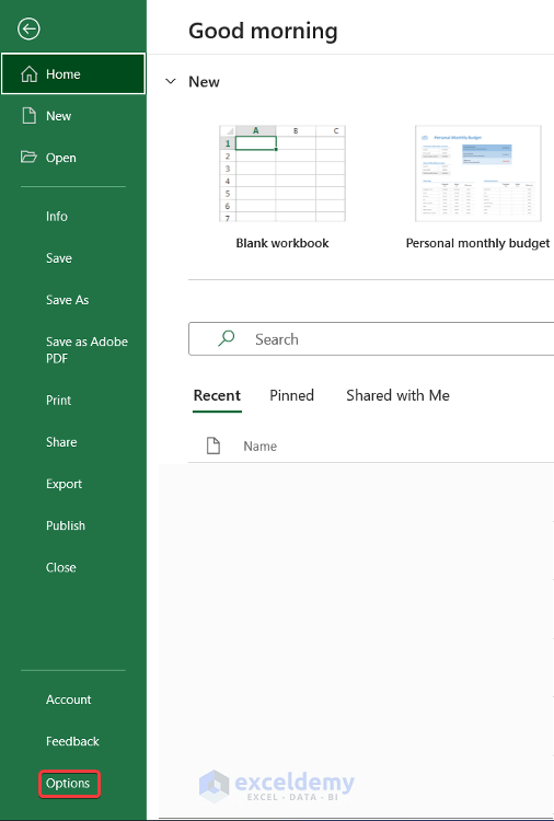
- A dialog box called Excel Options will appear.
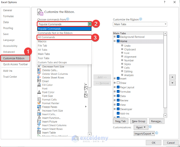
- Now, select the Customize Ribbon option.
- After that, select the drop-down arrow of the box below Choose commands from.
- Change the Popular Commands to All Commands option.
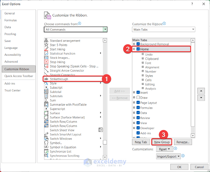
- All the commands of Excel will show below the box. Then, move down the slide bar of that box with the help of your mouse and find the Strikethrough command.
- Now, from the Main Tabs box, allocated on the right side, select your desired tab. We choose Home according to our desire.
- Next, click on the New Group option below the Main Tabs box.
- A new group titled New Group (Custom) will be created. Rename the group, if you want. Here, we keep the default group name.

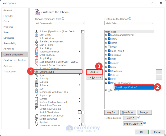
- Then, select the strikethrough command from the left box and click the Add button.
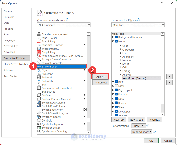
- You will see the command will add to the group entitled New Group.
- Finally, click OK.

- Now, select cell B8 and look at the far left side of the Home tab. You will find the group called New Group and the Srikethrough command.
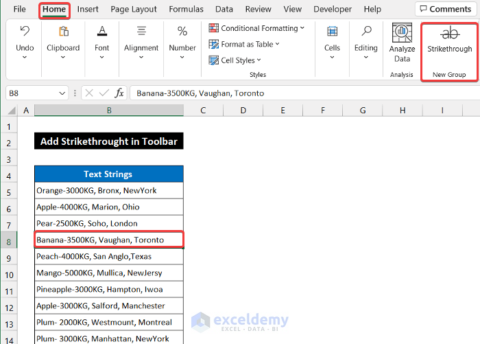
- Click on the command icon and you will get the Strikethrough format on cell B8.
Finally, we can say that according to our working steps, we are able to add the Strikethrough command in the Excel Toolbar.
Read More: How to Show Toolbar in Excel
2. Inserting Strikethrough in New Customized Tab
In this method, we will create a new tab and add the Strikethrough command from the Options into that tab. After that, we demonstrate the application to our dataset on cell B8. The steps of this approach are explained below:
📌 Steps:
- In the beginning, select File > Options.
- A dialog box entitled Excel Options will appear.
- After that, select the Customize Ribbon option.
- Then, select the drop-down arrow of the box below Choose commands from and change the Popular Commands to All Commands option.
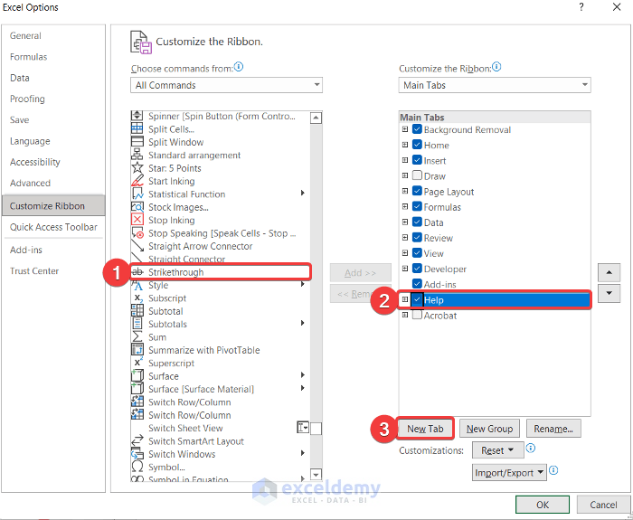
- You will see all the commands of Excel will show below the box. Now, move down the slide bar of that box and get the Strikethrough command.
- Now, from the Main Tabs box, allocated on the right side of the previous box, select any tab after which you want to insert the new tab. We choose Help as we want to place the new tab at last.
- Then, click on the New Tab option below the Main Tabs box.
- A new tab and group titled New Tab (Custom) and New Group (Custom) will be created. Rename them, if you want. Here, we keep the default names.
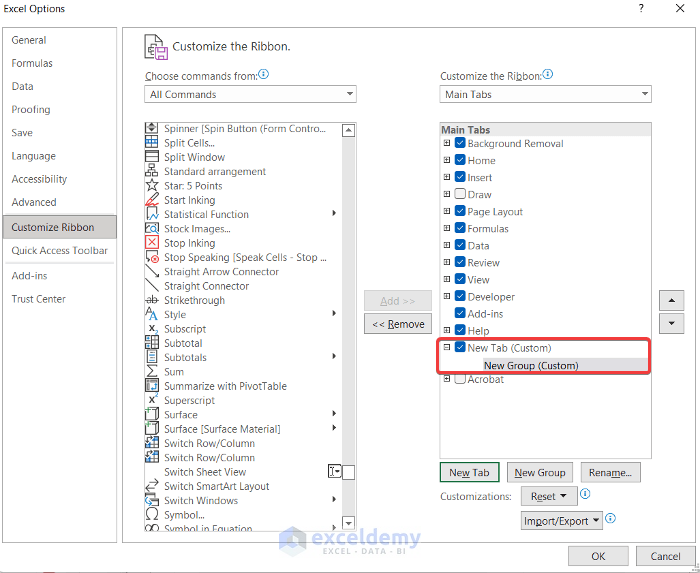
- Now, select the Strikethrough command from the left box, and after that New Group (Custom). Then, click the Add button.
- You will see the command will be added below the group name. At last, click OK to close the window.

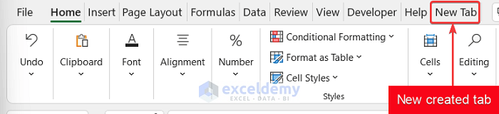
- You will see a new tab is created after the Help tab titled New Tab.
- Now, select cell B8, and in the New Tab, select the Strikethrough command from the New Group.
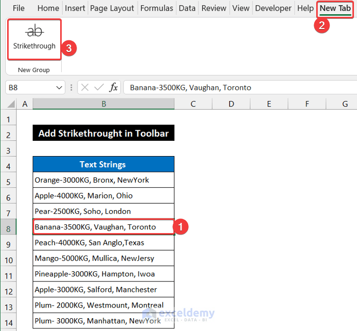
- You will get the Strikethrough format on cell B8.
Thus, we can say that our method worked successfully and we are able to add the Strikethrough command in Excel Toolbar.
3. Adding Strikethrough in Excel Quick Access Toolbar
Another way of showing the Strikethrough command in the toolbar is to add it to the Quick Access Toolbar. This toolbar is a separate toolbar from the Excel ribbon. It is usually located below or above the main Excel Ribbon. People usually add the most frequently used commands in that toolbar. In this method, we will show the procedure to add the Strikethrough command to the Quick Access Toolbar. The steps are given below:
📌 Steps:
- First, select File > Options.
- A dialog box entitled Excel Options will appear.
- Now, select the Quick Access Toolbar option.
- After that, select the drop-down arrow of the box below Choose commands from and change the Popular Commands to All Commands option.
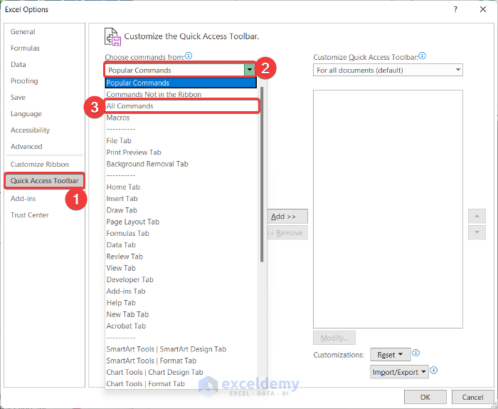
- All the commands of Excel will show below the box. Move down the slide bar of that box through your mouse to get the Strikethrough command.
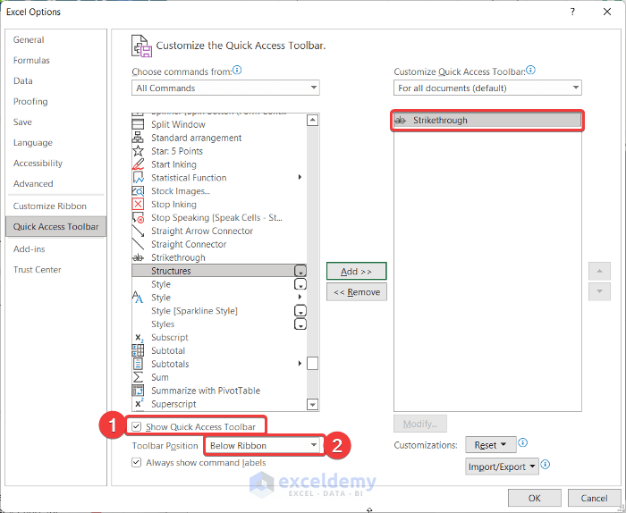
- Then, select the Strikethrough command, and click the Add button.

- The command will be added to the empty box on the right side.
- Below the All Commands box, check the Show Quick Access Toolbar option for displaying the toolbar. You can also choose the toolbar position by selecting the drop-down of the box titled Position. We choose the Below Ribbon option.
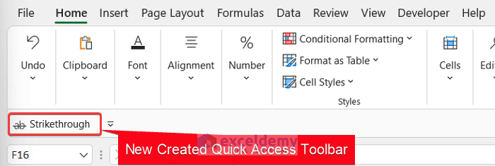
- Finally, click OK to close the window.
- You will see below the main Excel ribbon a new toolbar is created and it contains only the Strikethrough command.
- Now, select cell B8, and select the Strikethrough command from the Quick Access Toolbar.
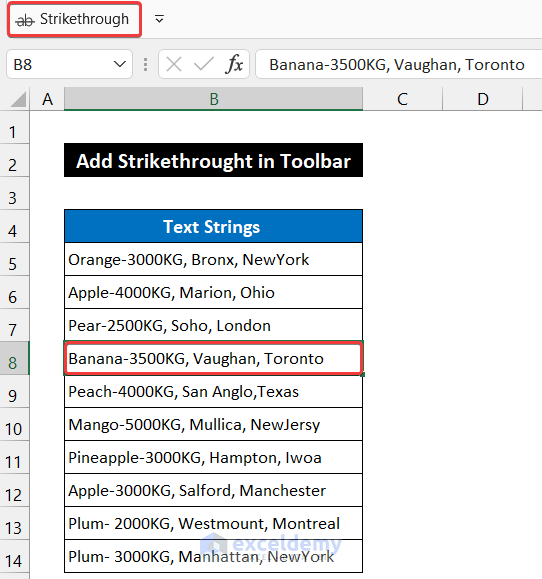
- You will see the Strikethrough format is applied on cell B8.
So, we can say that our method worked perfectly and we are able to add the Strikethrough command in the Excel toolbar.
Read More: How to Restore Toolbar in Excel
Download Practice Workbook
Download this practice workbook for practice while you are reading this article.
Conclusion
That’s the end of this article. I hope that this article will be helpful for you and you will be able to add the Strikethrough command in the Excel toolbar. If you have any further queries or recommendations, please share them with us in the comments section below.
Related Articles
<< Go Back to Toolbar in Excel | Excel Parts | Learn Excel
Get FREE Advanced Excel Exercises with Solutions!
