Conditional Formatting Based on Multiple Values of Another Cell

In this article, I’ll show you how you can apply Conditional Formatting in Excel based on multiple values of another cell. You’ll learn to apply Conditional Formatting on a single column and multiple columns, as well as on a single row or multiple rows, based on multiple values from multiple rows or columns. So, go through the entire article to get the full benefit.

Apply Conditional Formatting Based on Multiple Values of Another Cell in Excel: 4 Examples

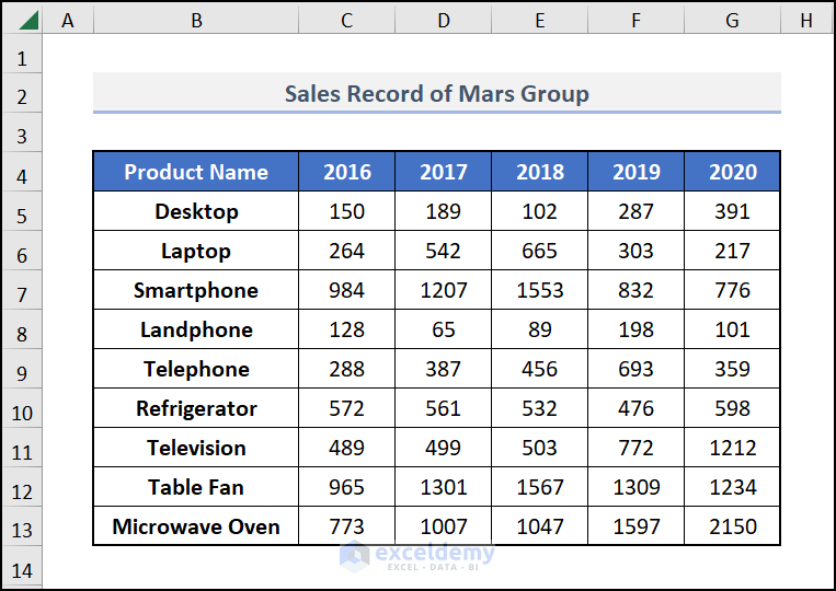
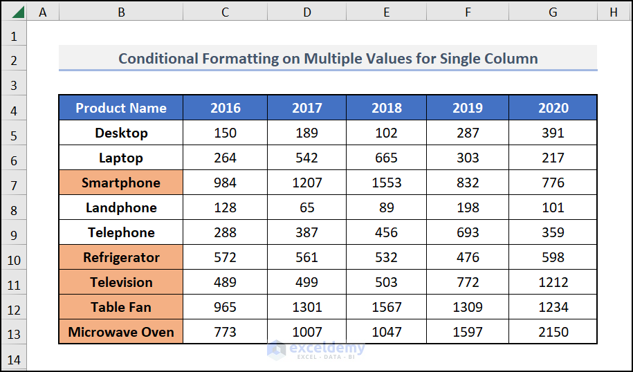
Here we’ve got a data Set with the sales record of some products for five years of a company named Mars group.

Today, our objective is to apply Conditional Formatting on this data set based on multiple values of another cell.

1. Conditional Formatting on a Single Column Based on Multiple Values of Another Cell

First of all, let’s try to apply Conditional Formatting on a single column based on multiple values of multiple cell in Excel.

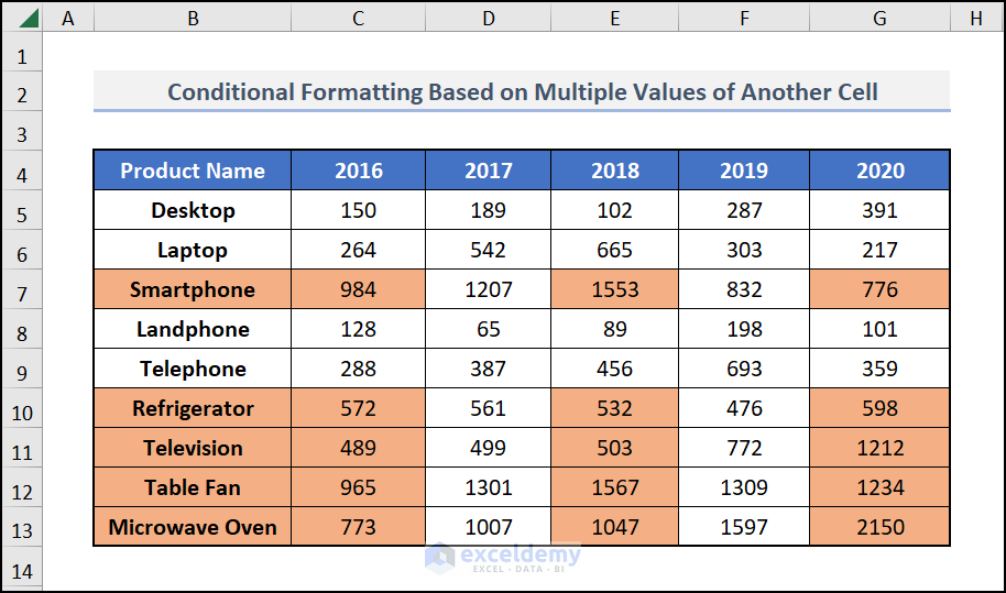
For example, let’s try to apply conditional formatting on the names of the products whose average sales in the five years are more than 500.

I am showing you the step-by-step procedure to accomplish this:

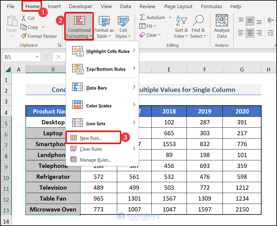
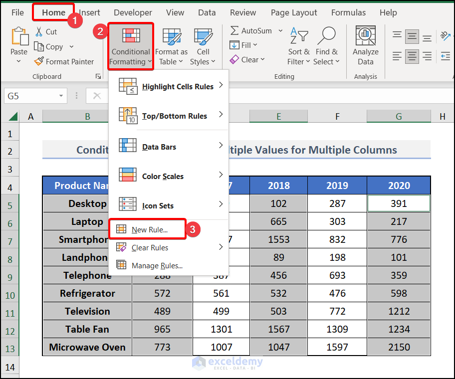
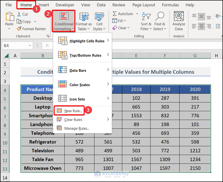
⧭ Step 1: Select Column and Open Conditional Formatting

• Firstly, select the column on which you want to apply Conditional Formatting.
• Then, go to the Home > Conditional Formatting > New Rule option in Excel Toolbar.

Here I’ve selected column B (Product Name).

⧭ Step 2: Insert Formula in New Formatting Rule Box

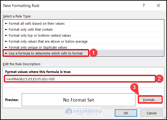
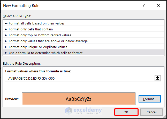
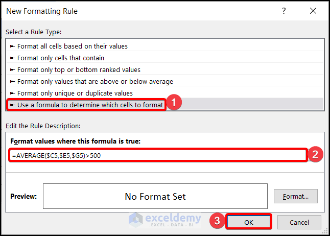
• Consequently, click on New Rule. You’ll get a dialogue box called New Formatting Rule.
• Subsequently, click on Use a formula to determine which cells to format. Insert the formula there:

or

⧪ Notes:

• Here, C5, D5, E5, F5, and G5 are the cell references of the first row, and AVERAGE()>500 is my condition. You use your own.
• When you apply Conditional Formatting on a single column based on multiple Values of another column, you can use either the Relative Cell References or the Mixed Cell References (Locking the Columns) of the cells, but not the Absolute Cell References.

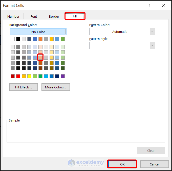
Sequentially, Click on Format. You’ll be directed to the Format Cells dialogue box.

• After that, from the formats available, choose the format you want to apply to the cells that fulfill the criteria.

I chose the light brown color from the Fill tab.

• Instantly, click on OK. You’ll be directed back to the New Formatting Rule dialogue box.

⧭ Step 3: Final Output

• Eventually, click on OK.

Finally, You’ll get the names of the products whose average sales are more than 500 marked in your desired format (Light brown in this example).

Read More: Conditional Formatting Based On Another Cell in Excel

2. Conditional Formatting on Multiple Columns Based on Multiple Values of Another Cell

You can also apply Conditional Formatting on multiple columns based on multiple values of multiple columns in Excel.

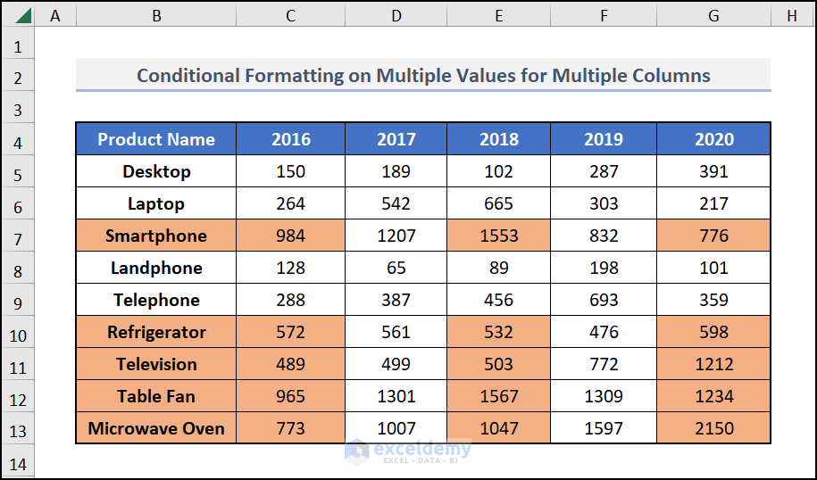
For example, let’s try to apply Conditional Formatting on the names of the products whose average in the years 2016, 2018, and 2020 are more significant than 500, along with the years.

The steps are the same as Example 1. In step 1, select all the columns on which you want to apply Conditional Formatting.

Here I’ve selected columns B, C, E, and G.

And in step 2, use the Mixed cell References (Locking the Columns) of the cells of the first row in the formula, not the Relative Cell References or the Absolute Cell References.

⧪ Note:

• When you apply Conditional Formatting on multiple columns based on multiple values from multiple columns, you must use the Mixed Cell References (Locking the Column).

Then choose the desired format from the Format Cells Dialogue Box. Then click on OK twice.

You will get the desired format applied to the cells of the multiple columns that fulfill your criteria.

⧪ More Example:

If you want, you can apply Conditional Formatting to the whole data set.

Just select the whole data set in step 1.

And apply the Mixed Cell References of the cells of the first row in the formula.

Then select the desired format and hit OK.

You’ll get cells of the whole data set that fulfill the criteria marked in your desired format.

Read More: Conditional Formatting Entire Column Based on Another Column in Excel

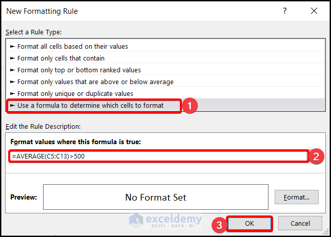
3. Conditional Formatting on a Single Row Based on Multiple Values of Another Cell

You can also apply Conditional Formatting on a single row based on multiple values of multiple rows in Excel.

For example, let’s try to apply Conditional Formatting to the years when the average sales of all the products were greater than 500.

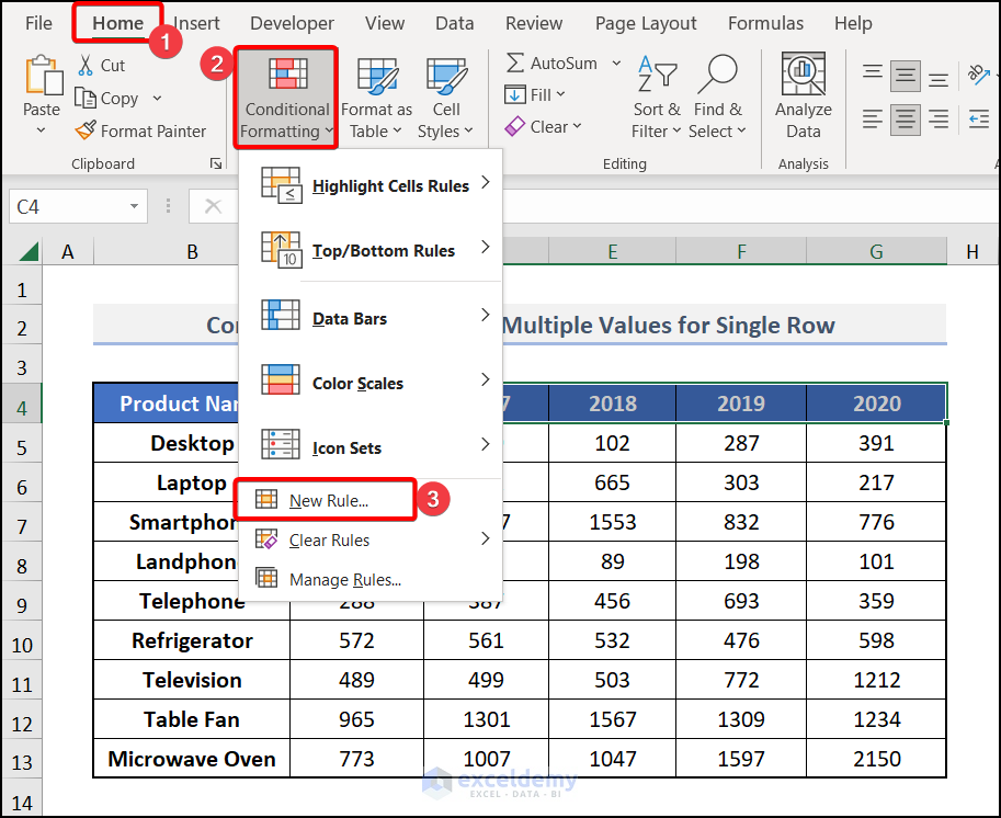
The steps are the same as Example 1. Just in step 1, select the row on which you want to apply Conditional Formatting.

Here I’ve selected C4:G4 (Years).

And in step 2, use the Relative Cell References or the Mixed cell References (Locking the Rows) of the cells of the first column.

or

⧪ Notes:

• Here, C5:C13 are the cell references of my first column. You use your one.
• When you apply Conditional Formatting on a single row based on multiple values from multiple rows, you must use either the Relative Cell References or the Mixed Cell References (Locking the Row).

Then choose the desired format from the Format Cells Dialogue Box. Then click on OK twice.

You will get the desired format applied to the years that had an average sales of more than 500.

Read More: Applying Conditional Formatting for Multiple Conditions in Excel

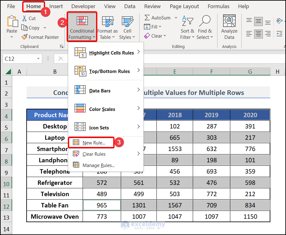
4. Conditional Formatting on Multiple Rows Based on Multiple Values of Another Cell

Finally, you can also apply Conditional Formatting on single rows based on multiple values of multiple rows.

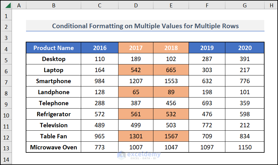
For example, let’s try to apply Conditional Formatting to the years, along with the sales when the average sales of the products Laptop, Landline, Refrigerator, and Table Fan were more than 500.

The steps are the same as Example 1. Just in step 1, select the rows on which you want to apply Conditional Formatting.

Here I’ve selected C4:G4, C6:G6, C8:G8, C10:G10, and C12:G12.

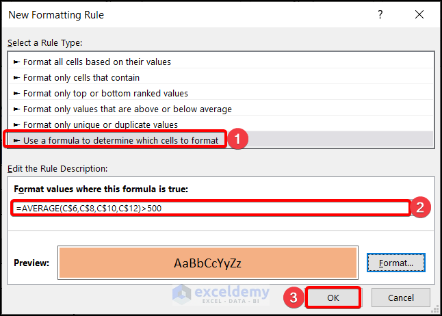
And in step 2, use the Mixed cell References (Locking the Rows) of the cells of the first column in the formula.

⧪ Note:

• When you apply Conditional Formatting on single rows based on multiple values from multiple rows, you must use the Mixed Cell References (Locking the Row).

Then choose the desired format from the Format Cells Dialogue Box. Then click on OK twice.

You will get the desired format applied to the cells that fulfill your condition.

Read More: How to Apply Conditional Formatting to Multiple Rows

How to Use Conditional Formatting with VBA Based on Another Cell

We can use VBA Conditional Formatting based on another cell value. Here, we will set the default color code to display the change. Follow the below steps to do it.

Steps:

• Initially, navigate to the Developer tab >> choose Visual Basic.

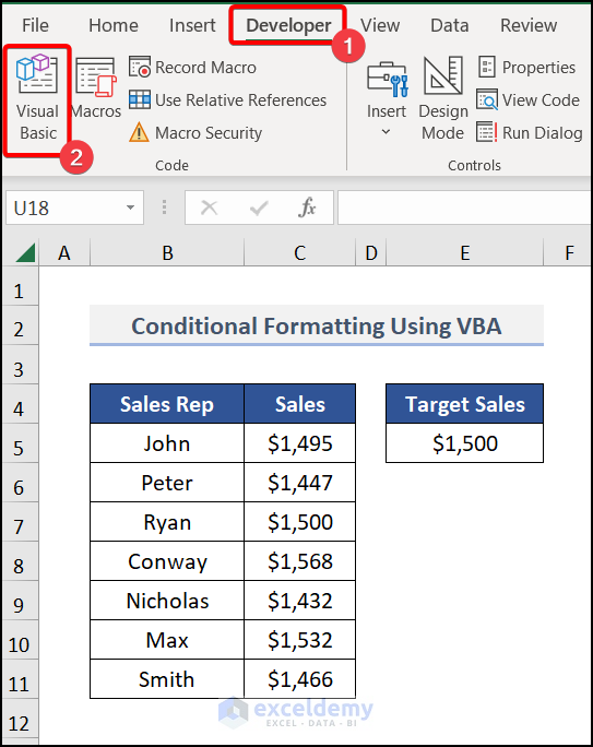
• Sequentially, go to the Insert tab in the Visual Basic Editor >> Module >> Module 1.

• Write up the following code in Module 1.

Sub ConditionalFormatting()
Dim RG As Range
Dim CD1 As FormatCondition
Dim CD2 As FormatCondition
Dim CD3 As FormatCondition
Set RG = Range("C5", Range("C5").End(xlDown))
RG.FormatConditions.Delete
Set CD1 = RG.FormatConditions.Add(xlCellValue, xlGreater, "=$E$5")
Set CD2 = RG.FormatConditions.Add(xlCellValue, xlLess, "=$E$5")
Set CD3 = RG.FormatConditions.Add(xlCellValue, xlEqual, "=$E$5")
With CD1
.Interior.Color = vbBlue
.Font.Color = vbWhite
End With
With CD2
.Interior.Color = vbRed
.Font.Color = vbWhite
End With
With CD3
.Interior.Color = vbYellow
.Font.Color = vbRed
End With
End Sub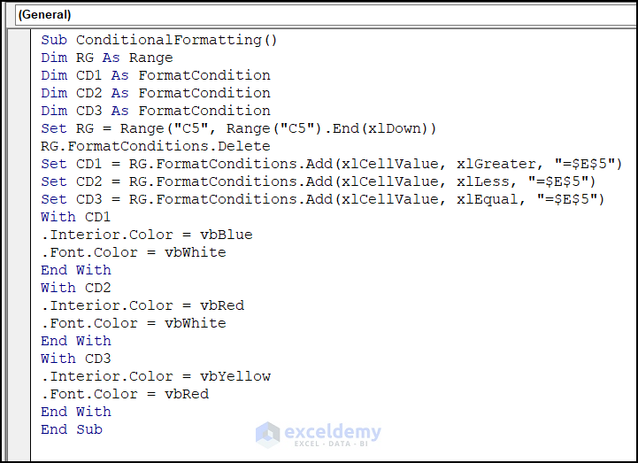

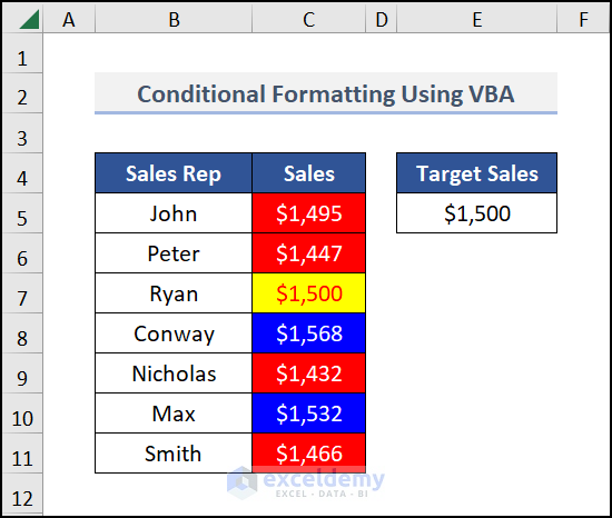
Run the code with the F5 key and get the following result.

Things to Remember

• While applying Conditional Formatting to a single column or multiple columns, insert a formula consisting of the cells of the first row.
• Similarly, while applying Conditional Formatting to a single row or multiple rows, insert a formula consisting of the cells of the first column.
• While applying Conditional Formatting on a single row or a single column, you can use either the Relative Cell References or the Mixed Cell References (Locking the column in the case of columns and locking the row in the case of rows.).
• But while applying Conditional Formatting on multiple rows or multiple columns, you must apply the Mixed Cell References.

Practice Section

We have provided a practice section on each sheet on the right side for your practice. Please do it by yourself.

Download Practice Workbook

Conclusion

That’s all about today’s session. These are some easy methods to use conditional formatting based on multiple values of another cell in Excel. Please let us know in the comments section if you have any questions or suggestions. For a better understanding please download the practice sheet.

Related Articles

• Change Font Color Based on Value of Another Cell in Excel
• How to Apply Conditional Formatting to the Selected Cells in Excel
  
• Conditional Formatting Based On Another Cell Range in Excel

<< Go Back to Conditional Formatting with Multiple Conditions | Conditional Formatting | Learn Excel