How to Use Sales Run Rate Formula in Excel (3 Handy Examples)

Sales run rate is an important parameter in the field of business, finance, e-commerce, and retail that wants to predict future revenue based on current sales performance. If you want to involve yourself in any of these sectors, you may need to make yourself familiar with how to calculate sales run rate. Obviously, Excel is a tool that will guide you with the most efficient steps. In this article, we have demonstrated the process of calculating sales run rate using a formula in Excel.

What Is the Sales Run Rate Formula?

The sales run rate is an indicator used to estimate a company’s potential future revenue based on its present revenue. It is determined by dividing the total current sales by the number of months that are involved with the current sales and then multiplying that value by 12. For instance, if a company makes $15,000 in sales in the first month of the year, its annual sales run rate ($15,000 x 12 months) is $180,000. If a company makes $5,000, $6,000, and $5,000 in sales in the first, second, and third months respectively of the year, their annual sales run rate (($5,000+6,000+5,000)/3) x 12 months) is $64,000.

Sales/Revenue Run Rate Formula:

We will be using the following formula in each of our examples.

How to Use Sales Run Rate Formula in Excel: 3 Suitable Examples

Sales run rate can be calculated based on various criteria. Here, we have explained the 3 most used cases of calculating sales run rate.

Example 1: Calculating Monthly Sales Run Rate

Suppose, the company you are working in has total sales of $15,000 in January. Now, you want to predict the annual total sales which is the sales run rate.

• Firstly, the total sales of January are displayed in Cell C7 in the following dataset.
• Select Cell C9, apply the formula below and press Enter–

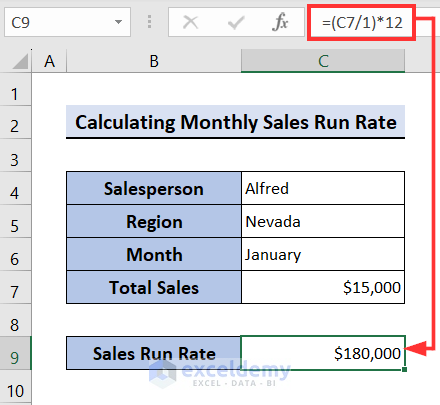
Example 2: Calculating Quarterly Sales Run Rate

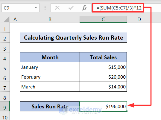
This time, your company has the total sales for January, February, and March. So, you have to calculate the quarterly sales run rate.

• Cell Range C5:C7 contains the total sales of January, February, and March.
• Select Cell C9, insert the formula below, and hit Enter–

As the formula of sales run rate mentioned earlier, the Current Sales are being calculated by SUM(C5:C7) and the number of months in the period here is 3.

Example 3: Calculating Half-Yearly Sales Run Rate

Assume, you have total sales from January to June. You have to calculate the half-yearly sales run rate.

• Select Cell C12 then apply the below formula.

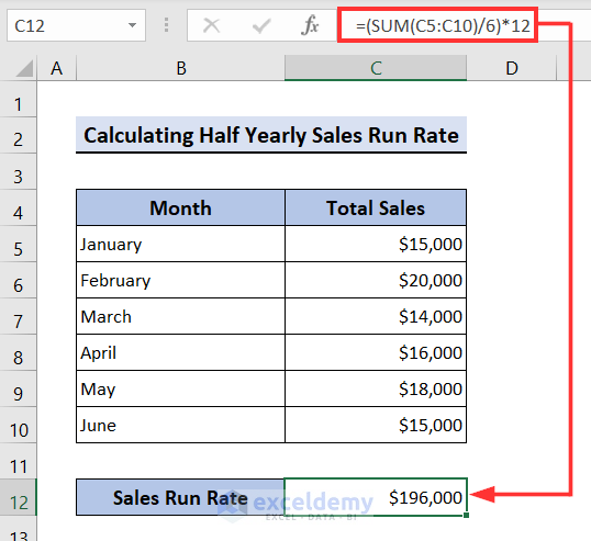
How to Calculate Dynamic Daily Run Rate in Excel

Let’s say, your company has to sell some products within March 31 meeting every product’s corresponding Plan Sales. Before March 10, each product’s Actual Sales are as follows. What you have to do is calculate each product’s daily run rate based on the total days left and based on working days left to meet the ultimate Plan Sales before the end of March.

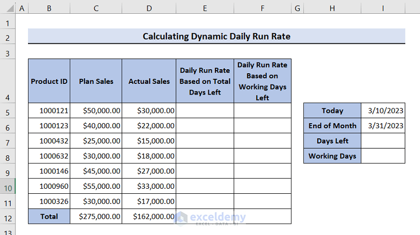
• First, let’s calculate the total days left. Here in Cell I5, we have inserted the starting date as March 10 as mm/dd/yyyy format which is 3/10/2023, and in Cell I6 end date is March 31 as 3/31/2023. Now, select Cell I7, and insert the formula below to calculate the total days left.

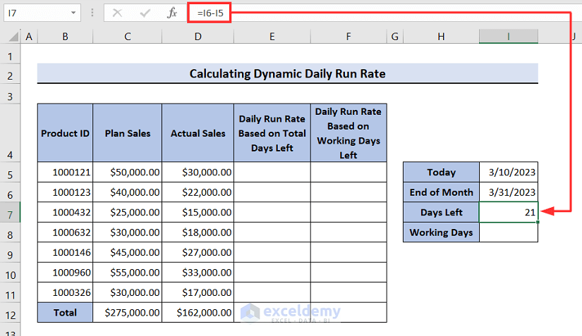
• To calculate the total working days left, you can use the NETWORKDAYS function. Select Cell I8, apply the formula below, and hit Enter–

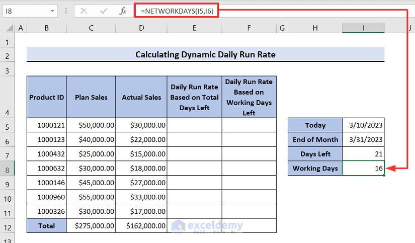
• Now, to calculate the daily run rate based on the total days left for the first product, select Cell E5, apply the formula below, and press Enter. After that, use the Fill handle icon to drag down.

• After dragging down the fill handle icon, you will get the daily run rate based on the total days left for the rest of the products as well. Now to determine the daily run rate based on working days left, simply select Cell F5, insert the formula below, and click on Enter. Again, use the Fill handle icon like previously.

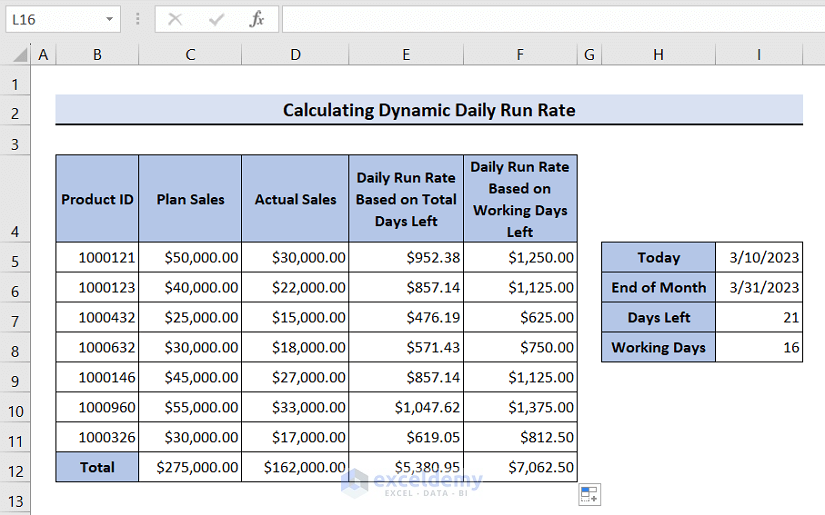
• After dragging down the fill handle icon, you will get the daily run rate of all the products based on the working days left as follows. Now, if you want to calculate the sum of the daily run rate of all the products, use the SUM function. Select Cell E12 then apply the formula below and press Enter. Use the Fill handle icon to drag right this time.

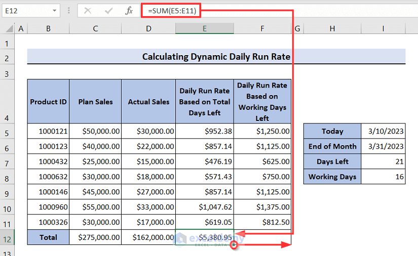
• Finally, a beautiful outcome of dynamic daily run rate you will get as follows.

How to Forecast Sales in Excel

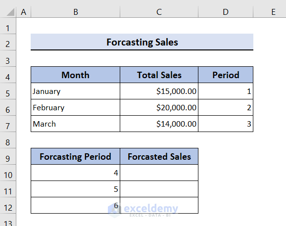
Using Excel’s FORECAST function is the simplest approach to forecast sales. Assume, you have data on total sales of January, February, and March and now you want to forecast sales for the next three months. Prepare the dataset as follows.

• Now, select Cell C10, apply the formula below, and press Enter. After that, use the Fill handle icon to drag down.

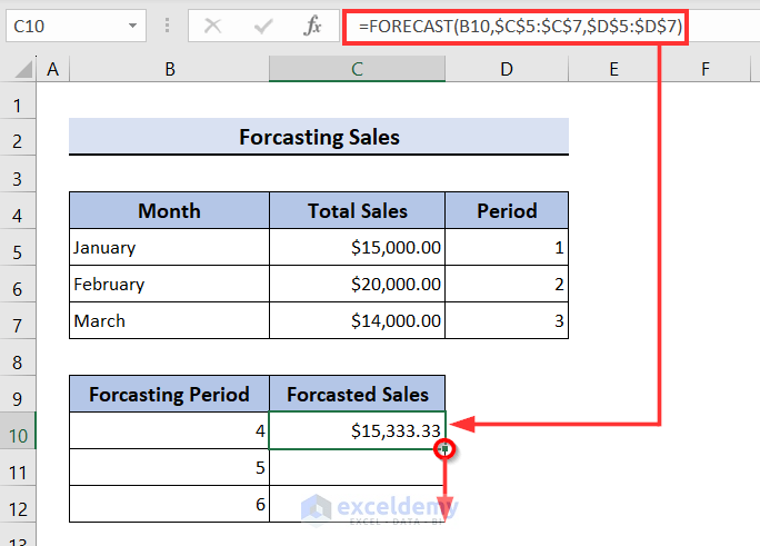
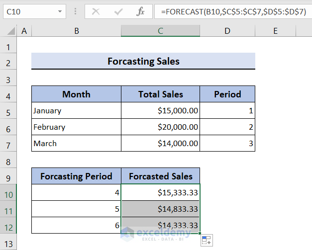
• Finally, you will get the forecasted sales for the next three months as follows.

Download Practice Workbook

Conclusion

Calculating sales run rate using a formula in Excel is an effective way of forecasting future sales using sales trends from the present. You may quickly determine your company’s sales run rate by following the instructions in this article, and you can use the results to guide key decisions about how to operate things in the future. Hope, this article will help you with whatever you are looking for. Visit our site ExcelDemy to explore more relevant articles that will surely make you more efficient and skillful in the world of Excel.

Frequently Asked Questions

1. How do you calculate the sales run rate in Excel?

The sales run rate can be calculated in Excel using the basic sales run rate formula which is-

Suppose, you have the total sales of January, February, and March in Cell A1, A2, and A3 respectively. Select an empty cell and apply the formula (SUM(A1:A3)/3)*12. This will return you the annual sales run rate.

2. What is a sales run rate?

The sales run rate is a forecast of the total revenue it expects to bring in over a specific time period based on its current sales trend. The business will earn sales at the same rate for the entire period, according to the projection. For instance, if a company makes $5,000 in sales in the first month of the year, its annual sales run rate ($5,000 x 12 months) is $60,000. If a company makes $5,000, $6,000, and $5,000 in sales in the first, second, and third months respectively of the year, their annual sales run rate (($5,000+6,000+5,000)/3) x 12 months) is $64,000.

3. How do I calculate running time in Excel?

Excel requires a start time and an end time to calculate running time in separate cells. The elapsed time is then obtained by subtracting the start time from the finish time. Suppose, the start time is in Cell A1 and the end time is in Cell B1.

Now, to calculate the number of hours between the start time and end time, select an empty cell and use this formula:

Remember, this will return 0 if the gap between the start and end time is less than 1 hour.

To calculate the number of hours and minutes between the two times use this formula:

To get hours, minutes, and seconds between those two times use this formula:

4. How do you calculate the sales formula?

The following equation can be used to determine the sales formula:

Here,

Units Sold: The total number of units sold over a specific time period.

Price per Unit: The cost of selling each unit.

5. How to forecast based on historical data?

The following formula can be used to forecast based on previous old data.

Here, x is the data point to be used to create a prediction.

known_ys is the dependent array or range of data (y values) known.

known_xs is the independent array or range of data (x values) is known.

<< Go Back to Sales | Formula List | Learn Excel