How to Use Excel SUMIF to Sum Values Greater Than 0 (3 Methods)

Introduction to the SUMIF Function in Excel

Microsoft Excel includes a built-in function called SUMIF, which allows you to add up values within a specified range based on specific conditions. This versatile function can be used to sum data based on either a single condition or multiple conditions.

The syntax for the SUMIF function is as follows:

SUMIF(range, criteria, [sum_range])

The arguments are as follows:

Arguments	Necessity	Value
range	Required	Refers to the range of cells you want to evaluate. The range of cells must be numbers, names, arrays, or references that have numbers. Blank and text values are ignored.
criteria	Required	Specifies the condition that determines which cells to include in the sum. The criteria can take the form of a number, expression, cell reference, text, or a function that specifies which cells should be included in the calculation.
sum_range	Optional	(Optional) Defines the range of cells whose values you want to sum. If omitted, the function will sum the values in the range. When determining which cells to add, we include cells other than those specified in the range argument. If the sum_range argument is omitted, Excel will sum the cells specified in the range argument.

When working with large datasets, the SUMIF function can be a powerful tool, helping you save time and effort.

Method 1 – Summing Values Greater Than 0 Using Criteria Inside Double Quotes in an Excel Formula

When utilizing the SUMIF function to calculate the sum of values greater than 0, you have the option to include the condition directly within the formula.

Scenario:
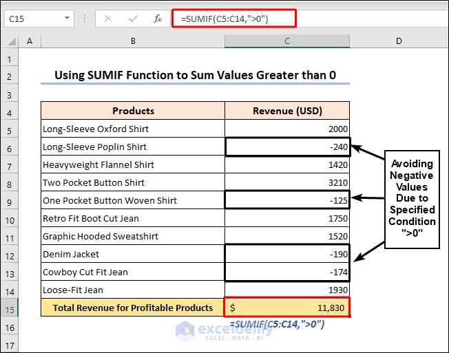
- You have a list of products that generated revenues over a period of time.
- Some products performed exceptionally well, while others fell short of expectations.
- Your goal is to calculate the sum of revenues for products that generated positive revenue and exclude those with negative revenue.

Formula:
- In cell C15, we inserted the following formula:

=SUMIF(C5:C14,">0")

- - The range argument (C5:C14) specifies the cells to evaluate.
  - The criteria argument (“>0”) defines the condition for inclusion (values greater than 0).

Result:
- Press Enter after entering the formula, and you’ll obtain the sum value.
- This sum includes only the revenues from products that exceeded 0.

Method 2 – Using the SUMIF Function When Criteria Range Differs

Suppose your sum range and criteria range are not the same. How do you modify your formula to calculate the sum for values greater than 0? In this section, we will discuss that scenario.

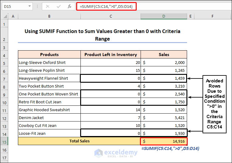
Let’s consider the example we’re using in this section. We have sales data for various products (located in cells D5:D14) and the corresponding inventory levels (in cells C5:C14). Our goal is to calculate the total sales, but only for items that are still in inventory. Specifically, we want to include products with positive inventory levels (greater than 0).

Formula:
- In cell D15, we inserted the following formula:

=SUMIF(C5:C14,">0",D5:D14)

- - The range argument (C5:C14) specifies the cells to evaluate based on a specific condition.
  - The criteria argument (“>0”) defines the condition (values greater than 0) and is enclosed in inverted commas (“”).

Explanation:
- The third argument is the range D5:D14, which contains the values to be summed based on the condition specified in the first argument.
- The formula will sum all the values in D5:D14, but only if the corresponding value in C5:C14 is greater than 0. If a value in the range C5:C14 is not greater than 0, it will be excluded from the sum.

Result:
- Press Enter after entering the formula, and you’ll obtain the sum value.

The SUMIF function provides an efficient way to perform such calculations when dealing with different criteria ranges.

[/wpsm_box]

Method 3 – Using Cell References for Criteria Values in Formulas

When you need a dynamic formula, consider using cell references instead of fixed values. Here’s how incorporating cell references can be helpful:

Scenario:
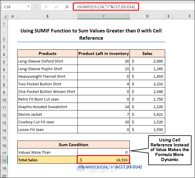
- We want to calculate the total sales for items that are still in inventory (i.e., where the quantity is greater than 0).
- Our criteria range is cells C5:C14, and the specified condition is “greater than 0.”

Formula:
- In cell C18, we insert the following formula:

=SUMIF(C5:C14,">"&C17,D5:D14)

Breakdown of the Formula:
- Range (C5:C14): This specifies the range of cells to assess based on the given condition.
- Criteria (“>” & C17): The “&” symbol concatenates the “>” symbol with the value in cell C17. This ensures that the function includes only values greater than the value in cell C17.
- Sum Range (D5:D14): These are the numbers to be summed up, based on the condition from the first argument.

Result:
- The formula sums all the values in D5:D14, but only if the corresponding value in C5:C14 is greater than the value in cell C17.
- To calculate the sum for values greater than any other value (except 0), simply change the value in cell C17 and press Enter.

Additional Notes:
- To include values less than 0, change the “>” operator to “<” (less than).
- To include values not equal to 0, use the “<>” operator within the formula.

How to Use the SUMIFS Function to Sum Values Greater than 0 in Excel

The SUMIF function is great for summing a range based on a single condition. However, when you need to apply multiple conditions, the SUMIFS function is your go-to choice.

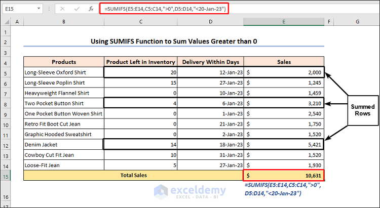
Here’s an example scenario: Suppose you want to calculate the total sales for items that are still in inventory and were delivered before January 20, 2023.

Formula:
- In cell E15, we insert the following formula:

=SUMIFS(E5:E14,C5:C14,">0",D5:D14,"<20-Jan-23")

Breakdown of the Formula:
- Range (E5:E14): This specifies the values to be summed based on the criteria from the second and third arguments.
- Criteria 1 (C5:C14, “>0”): The function evaluates the range C5:C14 based on the condition “>0”. Only values greater than 0 are included in the sum calculation.
- Criteria 2 (D5:D14, “<20-Jan-23”): This condition specifies that the function includes only values less than the date “20-Jan-23” in the sum.
- The formula sums all the values in E5:E14 that meet both conditions: greater than 0 and less than the specified date.

Result:
- Press Enter, and you’ll get the sum value.

Note: The main difference between the SUMIF and SUMIFS functions in Excel is the number of criteria that can be used. With SUMIFS, you can specify up to 127 pairs of criteria ranges and criteria.

Frequently Asked Questions

Can I Use the SUMIF Function to Calculate Values Greater Than 0 in a Range of Cells That Contains Errors or Empty Cells?
- If you want to exclude error values from the calculation, consider using the SUMIF function in combination with the IFERROR function. This allows you to replace error values with a 0. Typically, the SUMIF function ignores empty cells.
Can I Use the SUMIF Function with Non-Numeric Values?
- Yes, you can use the SUMIF function with non-numeric values. The function can sum up any values that meet the specified criteria, regardless of whether they are numeric or non-numeric. However, if you attempt to use the function with non-numeric values that cannot be converted to a number, it will return an error.
Can I Use Wildcards with the SUMIF Function?
- Absolutely! You can use wildcards such as asterisks (*) and question marks (?) with the SUMIF function. These wildcards allow you to match criteria based on partial text matches. Specifically:
  - The asterisk (*) represents any number of characters.
  - The question mark (?) represents a single character.