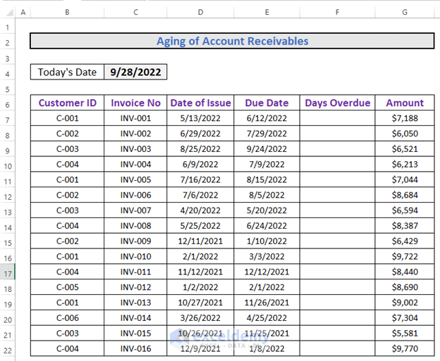
Here is the dataset for today’s article. There are some orders with due dates and amounts. We will calculate the Aging of Accounts Receivable using this dataset.
Method 1 – Apply the IF Function to Calculate the Aging of Accounts Receivable in Excel
Steps:
- Calculate the Days Overdue by inserting the following formula in F7:
=$C$4-E7- Press Enter to apply.
- Change the cell format to Number.
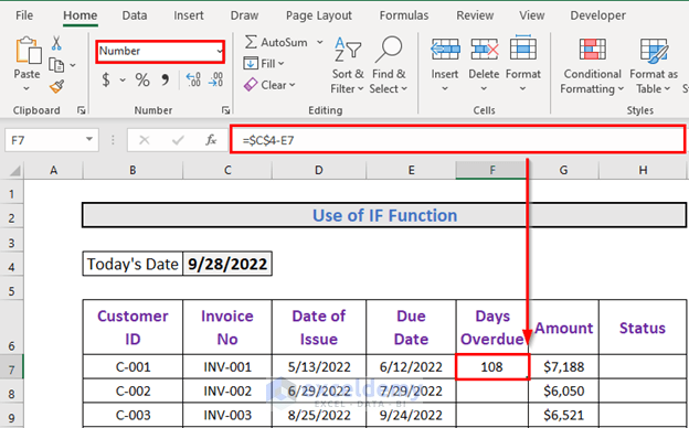
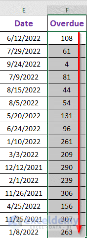
- Use the Fill Handle to AutoFill up to F22.
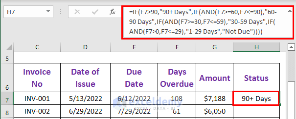
- To get the aging status, go to H7 and insert the following formula:
=IF(F7>90,"90+ Days",IF(AND(F7>=60,F7<=90),"60-90 Days",IF(AND(F7>=30,F7<=59),"30-59 Days",IF(AND(F7>0,F7<=29),"1-29 Days","Not Due"))))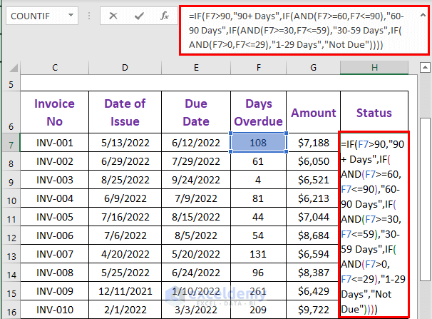
Formula Explanation:
The logical tests are:
- F7>90
- AND(F7>=60,F7<=90)
- AND(F7>=30,F7<=59)
- AND(F7>0,F7<=29)
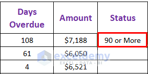
For F7 (108), the first test is TRUE. So, the corresponding output is 90+ Days.
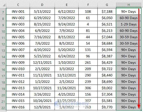
- Press Enter to get the output.
- AutoFill up to H22.
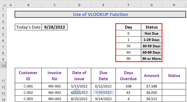
Method 2 – Use the VLOOKUP Function to Calculate the Aging of Accounts Receivable in Excel
We will modify the dataset a bit to include an aging table.
Steps:
- Go to H12 and insert the following formula:
=VLOOKUP(F12,$F$5:$G$9,2,TRUE)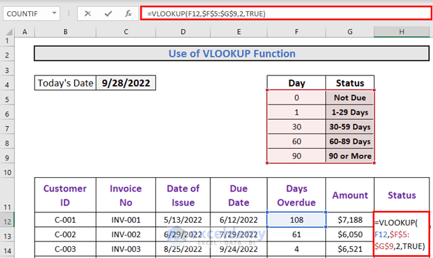
Formula Explanation:
- Excel will look for F12 in the array F5:G9.
- TRUE indicates that the match is an approximate one, not the exact one.
- 108 is the closest to 90. So the return is 90 or More.
- Press Enter to get the first result.
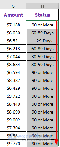
- Use the Fill Handle to AutoFill up to H27.
Method 3 – Apply the PivotTable Feature to Calculate the Aging of Accounts Receivable in Excel
Steps:
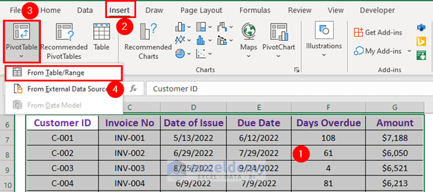
- Select the entire table.
- Go to the Insert tab.
- Select PivotTable.
- Choose From Table/Range.
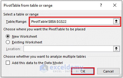
- A box will appear. Excel will automatically set the range. Click OK.
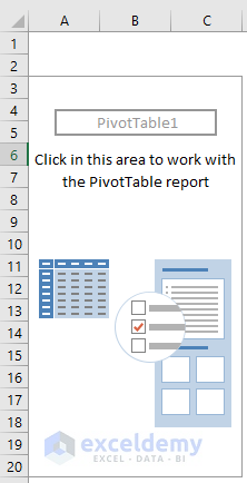
- Excel will create a PivotTable.
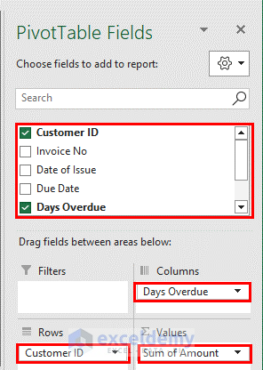
- From the PivotTable Fields, drag Customer ID to Rows, Days Overdue to Columns, and Amount to Values.
- Excel will, by default, show the sum of the amount.
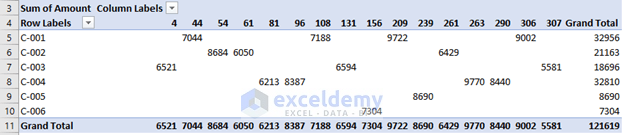
- You will get the following output.
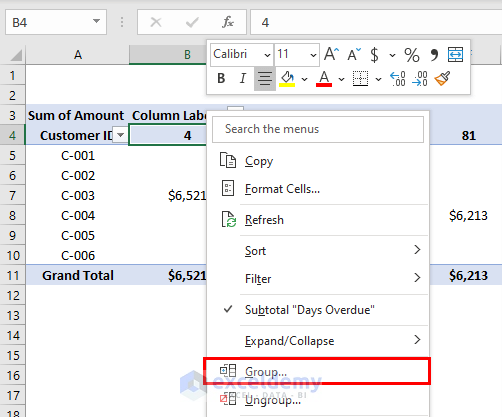
- To get the aging of accounts receivable, you have to group the Days Overdue.
- Select any cell from the row representing the Days Overdue.
- Right-click to get the context menu.
- Select Group.
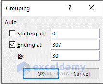
- A Grouping box will appear. Write 0 as the starting point.
- Keep 307 as the ending point.
- Use 30 as the grouping range.
- Click OK.
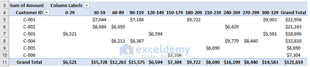
- Excel will return the aging of the accounts receivable.
Download the Practice Workbook
Download this workbook and practice while going through the article.
<< Go Back to Ageing | Formula List | Learn Excel
Get FREE Advanced Excel Exercises with Solutions!
