Color coding in Excel refers to the practice of assigning specific colors to cells or ranges of cells based on certain criteria or conditions. This visual formatting technique is a powerful tool for enhancing the readability of data within a spreadsheet.
In this Excel tutorial, you’ll learn step-by-step how to use conditional formatting to color code cells in Excel.
Why Is Color Coding Cells in Excel Important?
Color coding cells in your Excel spreadsheets can help visualize data, highlight important values, and make your files easier to analyze.
Here is a list of reasons why color coding cells may be important:
- Visual clarity: This can help you to distinguish between different categories or values, increasing readability.
- Pattern recognition: Colors help you identify patterns within the data, like understanding the different magnitudes of a spread of data.
- Highlighting exceptions: By assigning specific colors to cells that meet certain conditions, you can identify exceptions or outliers in the data.
- Customization for specific needs: You can tailor the color coding to suit their specific needs, whether it’s for financial analysis, project management, or any other type of data manipulation.
Color Code Cells with Conditional Formatting in Excel: Step-by-Step Guide
Conditional formatting is an extremely useful Excel feature that allows you to set rules that will automatically color cells based on their values.
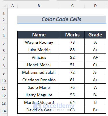
To showcase the process, we will use the following spreadsheet to color code the Marks column according to its values.
Here’s the step-by-step procedure to color code cells in Excel:
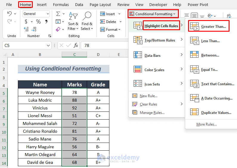
- Select the range of cells to color code.
- Go to the Home tab > Styles group > Conditional Formatting > Highlight Cell Rules > Greater Than….
 The Greater Than… option is selected to set the ‘greater than’ logical criteria. You can set this criteria according to your needs.
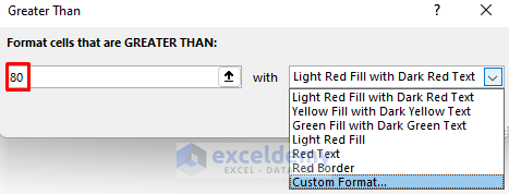
 - In the Greater Than dialog box:
- Input a value criteria.
The value has been set to 80 here in the Format cells that are GREATER THAN section. - Select the Custom Format… option from the ‘with’ drop-down menu.
- Input a value criteria.
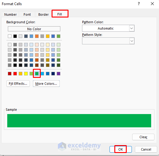
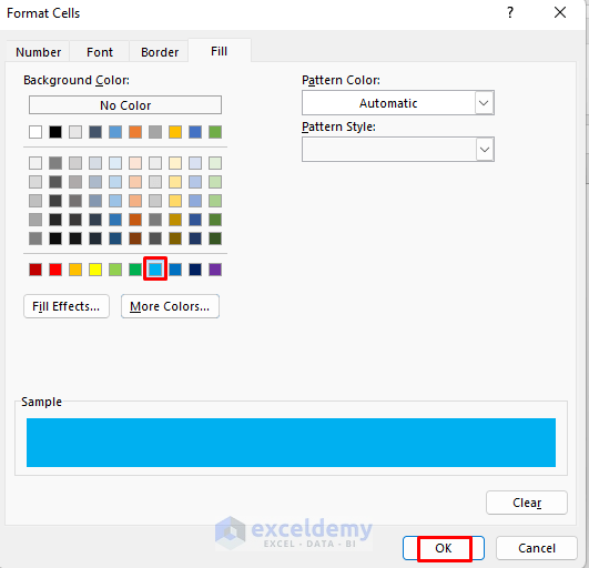
- In the Format Cells dialog box, go to the Fill tab
- Background Color > select desired fill color format > OK.
 Note: You can use all tabs (Number, Font, Border, and Fill) to apply different formatting.
 - Back in the Greater Than dialog box, press OK.
Here is the result of adding a color code to cells in Excel with conditional formatting.
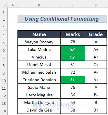
The color code criteria we have used here are the green background fill and white font color in the italics style.
2 Different Cases to Color Code Cells in Excel
Color coding cells in Excel can be beneficial in various scenarios to enhance data interpretation and analysis, especially in larger spreadsheets.
Here are 2 cases where you may need to color code in Excel:
Case 1: Color Cells Containing Excel Formulas
In larger spreadsheets, you may need to locate Excel formulas over a range of cells. Color coding with conditional formatting may serve as the best solution to highlight these cells.
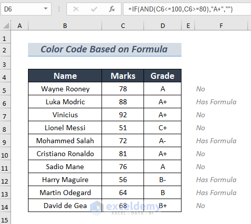
For example, in the following spreadsheet, some cells in the Grade column contain formulas. The best way to quickly find them is by using conditional formatting.
Here’s how you can color code cells containing formulas in Excel:
- Select the range of cells.
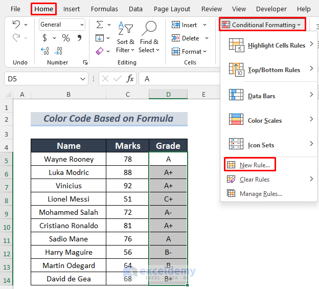
- Go to the Home tab > Styles group > Conditional Formatting > New Rule….
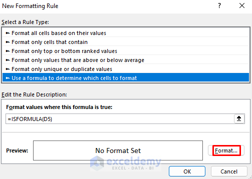
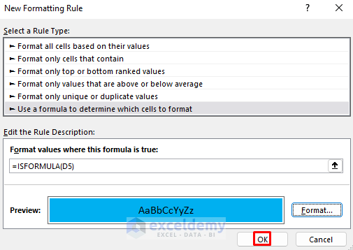
- In the New Formatting Rule dialog box:
- ‘Select a Rule Type:’ menu > ‘Use a formula to determine which cells to format’
- Under ‘Edit the Rule Description’, enter this conditioning formula:
=ISFORMULA(D5)
The formula uses the ISFORMULA function to address a formatting rule based on the formula, starting from cell D5. - Press Format….
- Set the desired format in the Format Cells dialog box > OK.
A shade of blue is selected as the background Fill color in this example.
- Back in the New Formatting Rule dialog box, click OK.
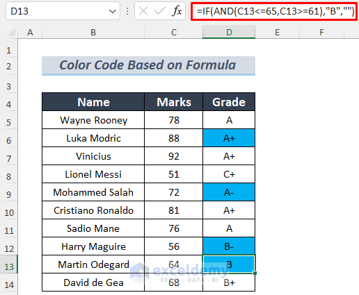
As a result, all the cells that match the criteria in the selected range have been color coded in Excel.
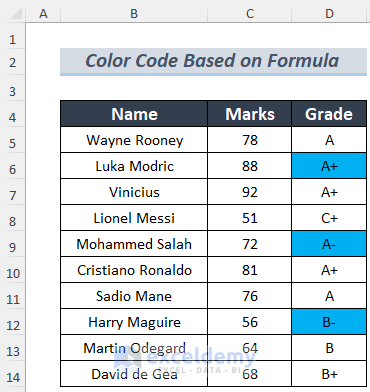
You can notice that if you apply a formula to another cell in that range, the cell also becomes color coded.
Case 2: Color Cells Based on Text Value
In larger spreadsheets, you may need to highlight cells containing specific text to easily identify them while scrolling. To that end, you can use conditional formatting to color code cells based on a text string in Excel.
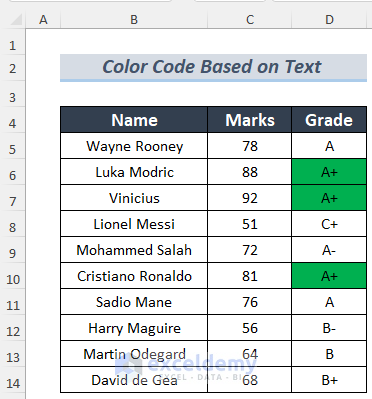
For example, in the following spreadsheet, the cells containing the string ‘A+’ in the Grade column will be highlighted.
Here is how we can color code cells based on text value in Excel:
- Select the range of cells.
- Go to the Home tab > Styles group > Conditional Formatting > New Rule….
- In the New Formatting Rule dialog box:
- ‘Select a Rule Type:’ menu > ‘Use a formula to determine which cells to format’
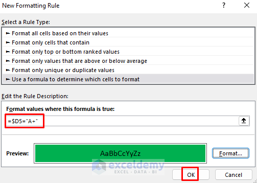
- Under ‘Edit the Rule Description’, enter this conditioning formula:
=$D5=”A+”
The formula checks for the string ‘A+’ starting from cell D5 and down the column. - Press Format….
- Set the desired format in the Format Cells dialog box > OK.
A shade of green is selected as the background Fill color in this example. - Back in the New Formatting Rule dialog box, click OK.
As a result, all the cells that match the criteria in the selected range have been color coded in Excel.
Download Practice Workbook
Conclusion
In conclusion, color coding cells in Excel is a practical and efficient way to visually organize and present data. And using Excel’s Conditional Formatting feature is the primary way to achieve this. Color coding cells in this way will facilitate you to better understand, analyze, and make decisions on large and complex datasets.
Feel free to leave any queries in the comments section below.
Frequently Asked Questions
Does Excel provide predefined color coding templates?
Yes, Excel offers predefined color coding templates through Conditional Formatting options like Color Scales, Data Bars, and Icon Sets. These templates provide quick solutions for common formatting needs.
Are there limitations to color coding in Excel?
While color coding is a powerful tool, excessive use may lead to visual clutter. Also, be cautious of potential color blindness issues, and ensure compatibility if sharing spreadsheets with others.
Related Articles
- Uses of CELL Color A1 in Excel
- VBA to Change Cell Color Based on Value in Excel
- How to Change Cell Color Based on a Value in Excel
- How to Fill Color in Cell Using Formula in Excel
- How to Fill Cell with Color Based on Percentage in Excel
- Excel Formula to Color Cell If It Has Specific Value
- How to Change Text Color with Formula in Excel
- How to Apply Formula Based on Cell Color in Excel
<< Go Back to Color Cell in Excel | Excel Cell Format | Learn Excel
Get FREE Advanced Excel Exercises with Solutions!
