Why It’s Actually Easier to Build Complex Filters in Power BI Than in Excel

 

When working with large datasets, filtering is one of the most powerful ways to focus on the information that matters. Both Excel and Power BI allow you to slice, dice, and drill down into data, but when it comes to complex filters, Power BI has a clear edge. Power BI is built with filtering in mind. Its filtering tools are intuitive, dynamic, and designed for scaling across multiple tables and millions of rows of data.

In this tutorial, we’ll explore why it’s actually easier to build complex filters in Power BI than in Excel.

The Pain Points of Complex Filters in Excel

Before exploring the power of Power BI, let’s acknowledge Excel’s strengths and shortcomings. Excel shines for small-to-medium datasets (up to about 1 million rows) and ad hoc analysis.

Basic Filters Are a Breeze:

• Select your data.
• Go to the Data tab >> select Filter.
• Check boxes for simple criteria.

Complex Filtering:

• Multi-Table Scenarios: Excel doesn’t natively handle relationships between sheets like a database. To filter across tables (e.g., sales data filtered by customer region from another sheet), you need VLOOKUP, INDEX-MATCH, or Power Query merges, which can bloat your file and slow performance.
• Dynamic or Conditional Filters: Consider you want to filter for “top 10 products by sales in Q1, but only if profit > 20%.” You can use an Advanced Filter, but it’s static and error-prone, or use formulas like SUMIFS or FILTER (in Excel 365). All of these approaches create a web of dependencies; change one thing, and something else breaks.
• Scalability Issues: With large data, Excel slows down. Filtering millions of rows? Expect lag, memory crashes, or “not responding” errors. Sharing interactive filters often means emailing massive files; recipients typically can’t tweak without the source data.

In short, Excel’s filters are linear and formula-heavy, making complex setups feel like manual labor.

Filtering in Excel

Suppose you want to find all West region orders with Sales >= 500, for multiple Categories. Here’s how to filter data in Excel.

Method 1: Using AutoFilter & Custom Filter

• Select your table range.
• Go to the Data tab >> select Filter.
  • Dropdown arrows will appear on headers.

• Click the Region column >> select only West.
• Click OK.

• Click the Sales Amount column >> click the dropdown >> select Number Filters >> select Greater Than Or Equal To….

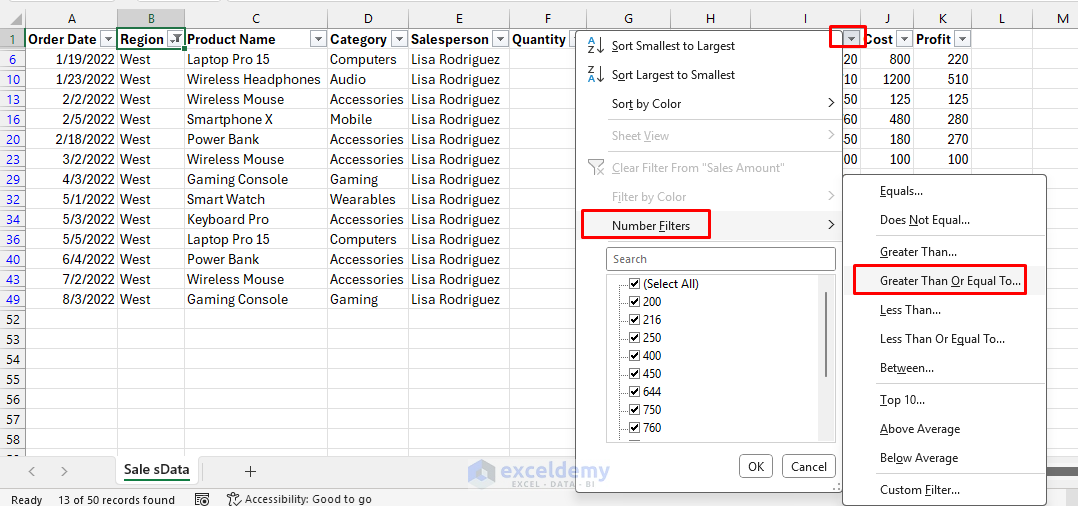
• Enter 500.
• Click OK.

• Click the Category column >> select Computers and Mobile.
• Click OK.

After applying all the filters one by one, you will get the desired result. Multiple filtering works, but this is manual. If your conditions change often, you must reapply filters every time.

Tip: If you create a table in Excel, it automatically enables the Filter option.

Method 2: Using Advanced Filter

• Copy headers (Region, Category, Sales Amount) to an empty area on the sheet.
• Enter the criteria for those columns.
• Select the original table.
• Go to the Data tab >> select Advanced.
  • Select Copy to another location.
  • Select the List range: A1:K51.
  • Select the Criteria range: M1:O3.
  • Select Copy to: M7.
• Click OK.

This works, but the criteria range setup is clunky and not dynamic. If you change the Region or Category, you must retype the conditions.

Method 3: Using the Dynamic FILTER Formula (Modern Excel)

Excel offers dynamic array formulas in recent versions; however, you will still require a solid understanding of functions and formulas.

• Select a cell and enter the following formula.

=FILTER(A2:K51,(B2:B51="West")*(I2:I51>=500)*((D2:D51="Computers")+(D2:D51="Mobile")))

• (B2:B51="West") ensures Region = West.
• I2:I51>=500 ensures Sales Amount >= 500.
• ((D2:D51="Computers")+(D2:D51="Mobile")) handles OR logic.

This FILTER formula is dynamic, but the expression can look intimidating to non-experts, and debugging multiple criteria can be painful.

Tip: PivotTable

You can use a PivotTable to filter, but it doesn’t offer flexible custom number filtering.

• Create a PivotTable.
  • Drag Region, Order Date, and Product Name to Rows.
  • Drag Category to Columns.
  • Drag Sales Amount to Values.
• Apply filters.
  • Select West from Row Labels.
  • Select Category from Column Labels.

Cons: Custom number filtering isn’t possible in a PivotTable.

Filtering in Power BI

Let’s apply the same filtering in Power BI using a similar dataset.

Method 1: Filters Pane

• Open Power BI Desktop.
• Load the dataset.
• Select Table from Visualizations.
  • Drag Order Date, Product Name, Region, Category, and Sales Amount to Columns.

• Go to the View tab >> select Filters.

• Open the Filters Pane (on the right side).
  • Expand Region in Filters >> choose West.
  • Click Apply filter.

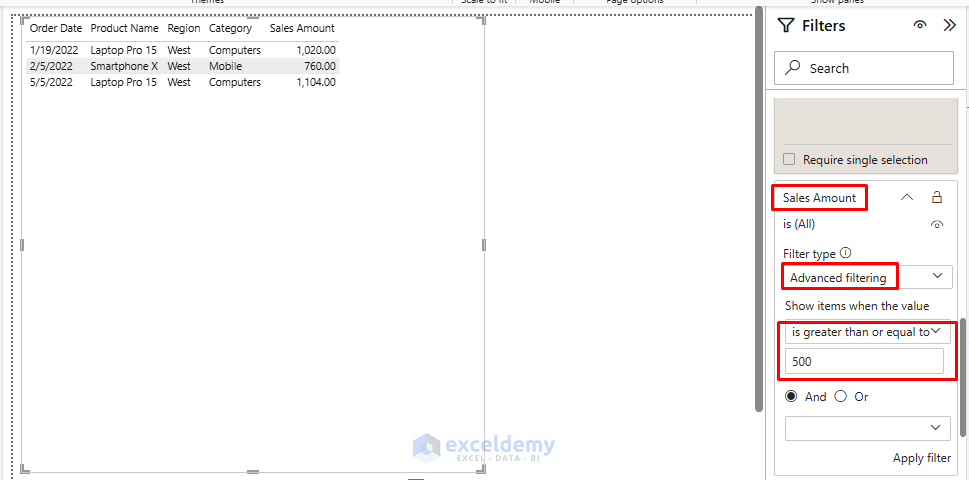
• Expand Sales Amount in Filters >> select Advanced filtering >> choose is greater than or equal to >> enter 500.
• Click Apply filter.

• Expand Category in Filters >> check Computers and Mobile.
• Click Apply filter.

• Power BI instantly filters the Table visual.

Method 2: Insert Visuals & Slicers (Interactive Filters)

• On the Report canvas, insert a Slicer visual.
  • Drag Region into Field and select West.
• Insert another Slicer.
  • Drag Category into Field and choose Computers and Mobile.
• Add a numeric slicer for Sales Amount.
  • Drag Sales Amount into Fields and set the minimum value to 500.
• Insert charts.
  • Pie chart to show Sales by Region.
  • Bar chart to show Sales by Products.
  • Line chart to show Monthly Trends.

• Now that the report is interactive, you can change conditions live without formulas.

Method 3: Page vs. Report vs. Visual Filters

• Visual Filter: Apply filters only to one chart.
  • Filter a Clustered Column chart to show the Top 5 products.

• Page Filter: Apply filters to all visuals on the same page.
  • The entire dashboard shows data for the West region.

• Report Filter: Apply filters across the whole report (all pages).
  • All pages will be filtered for the selected categories, Computers and Mobile.

• The filter is applied on another page as well.

This layered filtering is a core Power BI feature; Excel has no easy equivalent.

Why Power BI Is Easier

• No formulas are required—just checkboxes and sliders.
• Built-in AND/OR logic is handled automatically by filters.
• Dynamic visuals interactively change as conditions change.
• Scales to millions of rows; Excel struggles here.
• Reusable filtering: once set, filters apply across visuals and can be saved in reports.

Conclusion

Excel offers multiple ways to apply filters, but complexity increases as soon as you add AND/OR conditions, multiple columns, or dynamic criteria. Power BI makes the process much easier with its intuitive filter pane, slicers, and layered filters that scale with large datasets and update visuals in real time. Excel is powerful for quick, ad hoc analysis; it was never designed for managing complex, layered filters at scale. Power BI, on the other hand, was built specifically for interactive reporting and filtering. Based on your dataset and filter complexity, choose the best-suited platform.