The GETPIVOTDATA function runs a query across an entire pivot table and returns data based on its structure.
- Syntax
=GETPIVOTDATA (data_field, pivot_table, [field1, item1], …)
- Arguments
data_field: The name of the PivotTable field containing the data you want to return. This name must be enclosed in quotes.
pivot_table: The specific cell range containing the Pivot Table.
- Optional Arguments
field1, item1: The specific field and element names that you want to retrieve from the dataset, up to a maximum of 126 pairs. Non-numeric values must be enclosed in quotes.
Examples
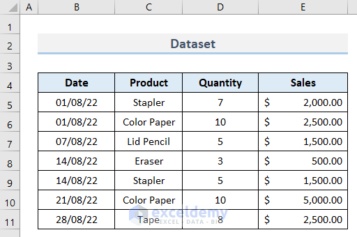
To describe the examples, we will create a pivot table first.
STEPS
- Create a dataset with the following information:
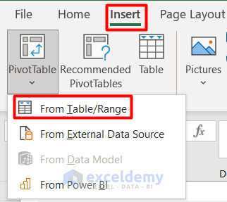
- Click the Insert tab.
- Select Pivot Table from the Tables group.
- Select From Table/Range from the drop-down section.
- Insert cell G4 as the Location – the pivot table will appear here.
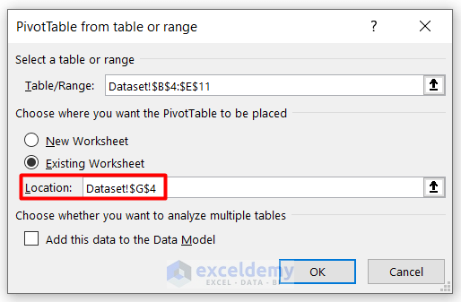
- Press OK.
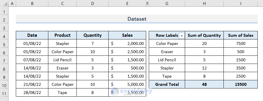
- The Pivot Table appears in the specified Location.
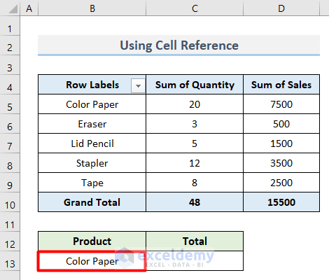
Example 1 – Use Excel Cell Reference with GETPIVOTDATA
We can use the GETPIVOTDATA function to extract a cell reference and return the required output.
STEPS
- Insert the name of the product in cell B13.
- Type an Equal (=) sign in cell C13.
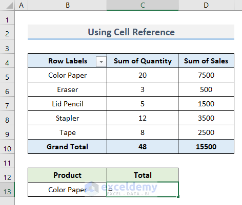
- Select cell D5, as it contains the Sales amount of our required product, Color Paper.
- Excel automatically generates the GETPIVOTDATA formula using the cell reference.
=GETPIVOTDATA("Sum of Sales",$B$4,"Product","Color Paper")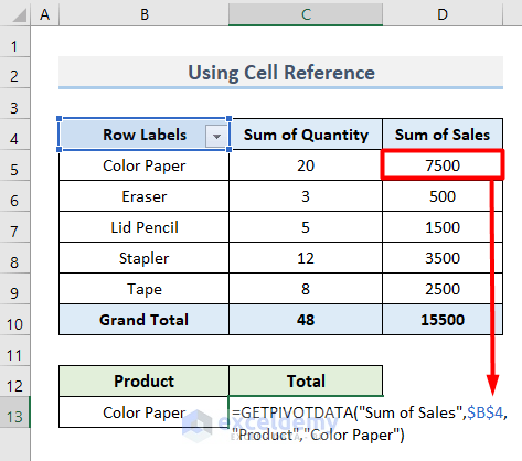
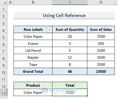
- Press Enter to return the final output.
Example 2 – GETPIVOTDATA in Cell References with a Value Field
If the pivot table has a value field, an additional Empty String must be concatenated onto the data_field parameter.
STEPS
- Insert this formula in cell C13 (as in Example 1):
=GETPIVOTDATA(B12&"",$B$4,"Product","Color Paper")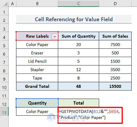
The reference cell B12 is associated with Empty String ( “” ) to concatenate the cell reference with cell B4.
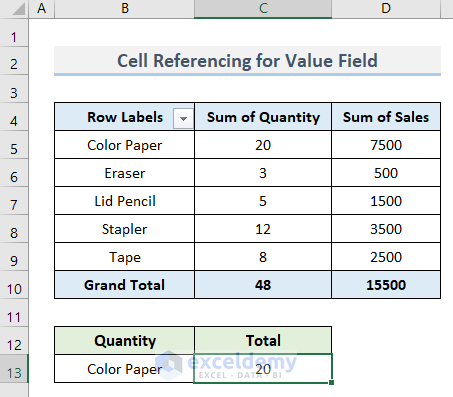
- Press Enter.
- The total sales amount of Color Paper is returned.
Example 3 – Insert Dates using GETPIVOTDATA
Here are four methods:
Method 3.1 – Match Date Format
To demonstrate, we will find the total amount of sales on 14/08/22.
similarDate is an important factor in running the function properly.
STEPS
- Insert the following formula in cell C13.
=GETPIVOTDATA("Sales",$B$4,"Date","14/08/22")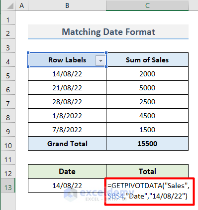
- Note – The same date format as the pivot table must be used.
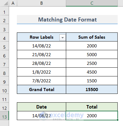
- Press Enter to return the result.
Method 3.2 – Apply DATEVALUE Function
Instead of typing manually, the DATEVALUE function can be used to filter or sort any dates in the pivot table if they are in text format.
To find the value of Product Quantity on 21/08/22:
STEPS
- Insert this formula in cell C13:
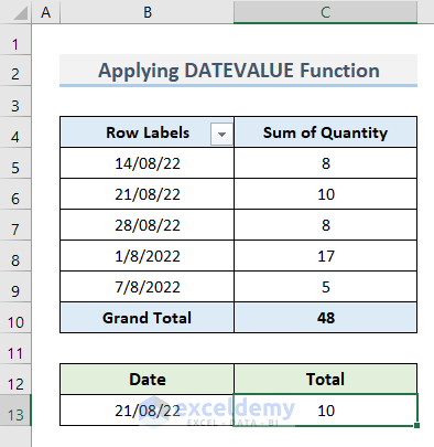
=GETPIVOTDATA("Quantity",$B$4,"Date",DATEVALUE("14/08/22"))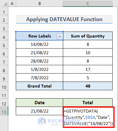
- Press Enter to return the result.
Method 3.3 – Insert DATE Function
The DATE function will be used to return the sequential serial number that represents the date in cell B13.
STEPS
- Insert this formula in cell C13:
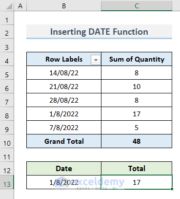
=GETPIVOTDATA("Quantity",$B$4,"Date",DATE(2022,1,8))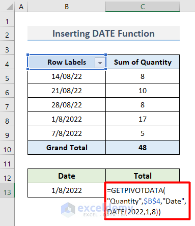
- Press Enter to return the result.
Method 3.4 – Use the TEXT Function
The TEXT function will be used to format the numbers given in the formula into date format, so that it runs correctly
STEPS
- Insert this formula in cell C13.
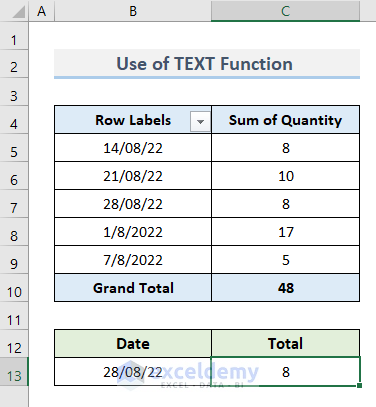
=GETPIVOTDATA("Quantity",$B$4,"Date",TEXT(B13,”dd/mm/yy”))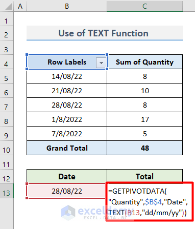
- Press Enter to return the result.
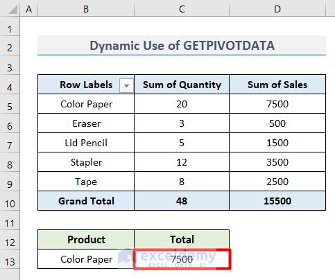
Example 4 – Dynamic Use of GETPIVOTDATA
Using the following procedure, output for any type of Product, rather than for a specific selected field, can be returned.
STEPS
- As in Example 1, the value of Sales for the product Color Paper is returned as follows:
- Insert this formula in cell B13, referencing the desired output cell:
=B9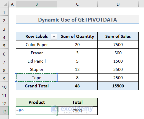
- Press Enter to return the result.
- The Total amount has been modified automatically, without the need for typing any formula.

How to Turn Off Auto Generation of GETPIVOTDATA in Excel
STEPS
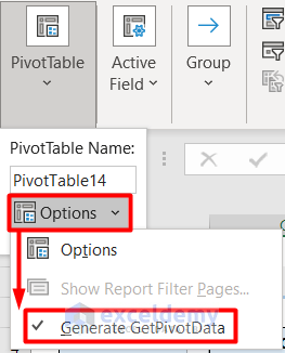
- Select any cell inside the Pivot Table.
- Click the PivotTable Analyze tab and select Pivot Table.
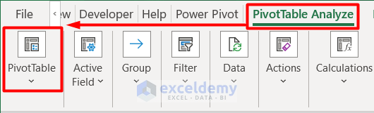
- Click on Options and de-select Generate GetPivotData.
Advantages
- Easy – it only takes one click on the reference cell to return the output.
- Flexible to modify at any stage.
Disadvantages
- Apart from the dynamic method, all the examples provided apply to single cells only, so the Autofill tool cannot be used to display multiple results.
Download Practice Workbook
How to Use GETPIVOTDATA in Excel: Knowledge Hub
<<Go Back to Pivot Table in Excel | Learn Excel
Get FREE Advanced Excel Exercises with Solutions!
